Understanding Top 10 Classical Machine Learning Algorithms
Before jumping into Deep Learning, one must know the classical/traditional Machine Learning algorithms, because understanding traditional machine learning algorithms can provide a strong foundation in machine learning concepts. These algorithms often involve simple, intuitive concepts that can be helpful in understanding more complex deep learning models.
Traditional machine learning algorithms can be faster to train and easier to interpret than deep learning models. This can be particularly useful in situations where you need to make quick decisions or where it's important to understand the reasoning behind a model's predictions. Traditional machine learning algorithms can be more effective for certain types of problems. For example, linear models like linear regression and logistic regression can be effective for problems with a small number of features, while decision trees and random forests can be effective for problems with a large number of features.
Deep learning algorithms can be more difficult to learn and require a lot of data and computational resources to train effectively. By learning traditional machine learning algorithms first, you can get a sense of how different algorithms work and what types of problems they are best suited for, which can make it easier to decide when and how to use deep learning algorithms.
Linear Regression
Linear regression is a machine learning algorithm used for modeling the linear relationship between a dependent variable (also known as the target or output variable) and one or more independent variables (also known as the features or input variables). It is used to make predictions about the value of the dependent variable based on the values of the independent variables.
In univariate linear regression, there is only one independent variable, while in multivariate linear regression, there are multiple independent variables (also known as features).
The line that is fit to the data in linear regression is defined by the equation
1y = mx + b
where y is the dependent variable, x is the independent variable, m is the slope of the line, and b is the y-intercept (the point where the line crosses the y-axis).
In the context of machine learning, this equation can be written as
1h(X) = W0 + W1.X
where W0 and w1 are weights, X is the input feature, and h(x) is the label (i.e. y-value).
The goal of linear regression is to find the weights (W0 and w1) that lead to the best-fitting line for the input data. The best-fitting line is determined in terms of the lowest cost, which is a measure of how far off the model's predictions are from the actual training data. Linear Regression, The Mean Squared Error (MSE) loss function is used usually.
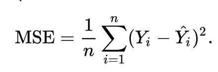
Essentially, the MSE measures the average of the squared residuals (the difference between actual and predicted values). To get a more intuitive understanding, let’s dive deeper into what each variable means.
- Y = the actual data point
- ŷ (pronounced y hat) = the predicted data point
- n = the total amount of data points
Training a linear regression model involves using a learning algorithm to find the weights (w0 and w1) that minimize the cost. One common algorithm used for this purpose is gradient descent, which involves iteratively updating the values of w0 and w1 in the direction that minimizes the cost. The algorithm follows the following pseudo-code:
1Repeat until convergence {
2    temp0 := W0 - a.((d/dW0) J(W0,W1))
3    temp1 := W1 - a.((d/dW1) J(W0,W1))
4    W0 = temp0
5    W1 = temp1
6}
Where (d/dW0) and (d/dW1) are the partial derivatives of J(W0,W1) with respect to W0 and W1, respectively. The gist of this partial differentiation is basically the derivatives:
1(d/dW0) J(W0,W1) = W0 + W1.X - T
2(d/dW1) j(W0,W1) = (W0 + W1.X - T).X
If we run the gradient descent learning algorithm on the model, the model will converge to a minimum cost. The weights that led to that minimum cost are used as the final values for the line function h(x) = w0 + w1x, which is the linear regressor.
Once the model is trained, it can be used to make predictions about the dependent variable for new data by plugging in the values of the independent variables into the equation of the line. The performance of the model can be evaluated by comparing the predicted values to the actual values of the dependent variable in.
Read more about the different types of regression models from here in this blog.
Implementation
 1from sklearn.model_selection import train_test_split
 2from sklearn.linear_model import LinearRegression
 3from sklearn.metrics import mean_absolute_error, mean_squared_error, r2_score
 4
 5
 6
 7# Split the data into training and test sets
 8X_train, X_test, y_train, y_test = train_test_split(X, y, test_size=0.2, random_state=42)
 9
10# Scale the features (optional)
11from sklearn.preprocessing import StandardScaler
12scaler = StandardScaler()
13X_train = scaler.fit_transform(X_train)
14X_test = scaler.transform(X_test)
15
16
17# Create the linear regression model
18model = LinearRegression()
19
20# Fit the model to the training data
21model.fit(X_train, y_train)
22
23# Make predictions on the test data
24y_pred = model.predict(X_test)
25
26# Calculate the mean absolute error (MAE)
27mae = mean_absolute_error(y_test, y_pred)
28
29# Calculate the mean squared error (MSE)
30mse = mean_squared_error(y_test, y_pred)
31
32# Calculate the root mean squared error (RMSE)
33rmse = np.sqrt(mse)
34
35# Calculate the R2 score
36r2 = r2_score(y_test, y_pred)
Polynomial Regression
Polynomial regression is a type of regression analysis in which the relationship between the independent variable x and the dependent variable y is modeled as an n-th degree polynomial. It is used to model relationships between variables that are not linear.
Fig: Linear Regression [3]
Fig: Polynomial Regression [3]
Polynomial regression is a type of regression analysis in which the relationship between the independent variable x and the dependent variable y is modeled as an nth degree polynomial. Polynomial regression can be used to model relationships between variables that are not linear.
Linear regression models the relationship between two variables using a straight line. But sometimes the relationship between two variables is more complex, and a straight line is not the best way to model this relationship. In these cases, polynomial regression can be used.
To perform polynomial regression, you first need to choose the degree of the polynomial that you want to fit to the data. The degree of the polynomial determines the number of curvatures in the line. A polynomial of degree 1 is a straight line, while a polynomial of degree 2 has one curvature, and so on.
Once you have chosen the degree of the polynomial, you can then fit the model to the data by finding the coefficients of the polynomial that minimize the sum of the squared errors. The coefficients of the polynomial are then used to predict the value of y for a given value of x.
One of the main differences between linear and polynomial regression is the shape of the curve that is fit to the data. Linear regression fits a straight line to the data, while polynomial regression can fit curves of any degree. This makes polynomial regression more flexible and able to model more complex relationships between variables.
Another difference between linear and polynomial regression is the way that they handle outliers. Outliers are data points that are significantly different from the rest of the data. In linear regression, outliers can have a large influence on the slope of the line, which can result in an inaccurate model. However, in polynomial regression, the curve is able to bend and adapt to the outliers, which can result in a more accurate model.
Polynomial regression can be a powerful tool for understanding and predicting complex relationships between variables. However, it is important to be careful when using polynomial regression, as it can be prone to overfitting. Overfitting occurs when the model is too complex and fits the noise in the data rather than the underlying trend. This can result in a model that is accurate for the training data, but performs poorly on new data. To avoid overfitting, it is important to choose the appropriate degree of the polynomial and to use cross-validation to assess the performance of the model.
Implementation
 1from sklearn.model_selection import train_test_split
 2from sklearn.preprocessing import PolynomialFeatures
 3from sklearn.linear_model import LinearRegression
 4
 5
 6# Split the data into training and test sets
 7X_train, X_test, y_train, y_test = train_test_split(X, y, test_size=0.2, random_state=42)
 8
 9# Scale the features (optional)
10from sklearn.preprocessing import StandardScaler
11scaler = StandardScaler()
12X_train = scaler.fit_transform(X_train)
13X_test = scaler.transform(X_test)
14
15# use the PolynomialFeatures class to transform the independent variables into polynomial features
16poly = PolynomialFeatures(degree=2)
17X_train_poly = poly.fit_transform(X_train)
18X_test_poly = poly.transform(X_test)
19
20# Create the linear regression model
21model = LinearRegression()
22
23# Fit the model to the training data
24model.fit(X_train_poly, y_train)
25
26# Make predictions on the test data
27y_pred = model.predict(X_test_poly)
Logistic Regression
Logistic regression is a statistical method used for predicting the probability of a binary outcome. It is a type of regression analysis that is used when the dependent variable is dichotomous, or has only two possible values. Logistic regression is often used in fields such as marketing, finance, and psychology to predict the likelihood of an event occurring, such as whether a customer will purchase a product or whether a patient will respond to a treatment.
Linear regression is a statistical method that is used to model the linear relationship between a dependent variable and one or more independent variables. It is used to predict a continuous outcome, such as the price of a house or the amount of rainfall in a given year.
One of the main differences between logistic regression and linear regression is the type of dependent variable that they are used to model. Logistic regression is used to model dichotomous variables, while linear regression is used to model continuous variables.
Another difference between logistic regression and linear regression is the way that the models are fit to the data. In linear regression, the model is fit by minimizing the sum of the squared errors between the predicted values and the actual values. In logistic regression, the model is fit by maximizing the likelihood of the observed data, given the model. This is done using an optimization algorithm, such as gradient descent.
To perform logistic regression, you first need to choose the independent variables that you want to include in the model. These variables should be chosen based on their relevance to the outcome that you are trying to predict. The logistic regression model is then fit to the data by estimating the coefficients of the independent variables. The coefficients represent the effect of each independent variable on the probability of the outcome occurring.
Once the model has been fit to the data, it can be used to make predictions about the probability of the outcome occurring for a given set of values of the independent variables. The predicted probability can be transformed into a binary prediction by setting a threshold value. For example, if the threshold is set at 0.5, then any predicted probability greater than 0.5 is classified as a positive outcome, while any predicted probability less than 0.5 is classified as a negative outcome.
When not use Logistic regression
There are several situations when logistic regression may not be the best choice for analyzing data:
- When the dependent variable is not binary: Logistic regression is only suitable for predicting the probability of a binary outcome, such as whether an event will occur or not. If the dependent variable has more than two categories, logistic regression is not appropriate.
- When the independent variables are not independent: Logistic regression assumes that the independent variables are independent of each other. If there are strong correlations between the independent variables, the model may be biased and produce inaccurate results.
- When the data is imbalanced: Logistic regression is sensitive to class imbalances, where one class is much more prevalent than the other. This can lead to poor performance of the model on the minority class.
- When the data has non-linear relationships: Logistic regression is a linear model, so it may not be suitable for data that has non-linear relationships. In these cases, a non-linear model such as decision trees or support vector machines may be more appropriate.
- When the sample size is small: Logistic regression is prone to overfitting when the sample size is small. This means that the model may perform well on the training data, but poorly on new data. To avoid overfitting, it is important to have a large enough sample size to accurately estimate the coefficients of the model.
Implementation
 1from sklearn.linear_model import LogisticRegression
 2from sklearn.model_selection import train_test_split
 3import pandas as pd
 4from sklearn.metrics import accuracy_score, precision_score, recall_score
 5
 6
 7# Load the data into a Pandas DataFrame
 8df = pd.read_csv("data.csv")
 9
10# Split the data into features and target variables
11X = df.drop("target", axis=1)
12y = df["target"]
13
14# Split the data into training and testing sets
15X_train, X_test, y_train, y_test = train_test_split(X, y, test_size=0.2)
16
17# Create an instance of the LogisticRegression class
18model = LogisticRegression()
19
20# Fit the model to the training data
21model.fit(X_train, y_train)
22
23# Make predictions on the testing data
24y_pred = model.predict(X_test)
25
26# Calculate the accuracy of the model
27accuracy = accuracy_score(y_test, y_pred)
28
29# Calculate the precision of the model
30precision = precision_score(y_test, y_pred)
31
32# Calculate the recall of the model
33recall = recall_score(y_test, y_pred)
34
35print("Accuracy:", accuracy)
36print("Precision:", precision)
37print("Recall:", recall)
Support Vector Machines (SVM)
Support Vector Machines (SVMs) are a type of supervised learning algorithm that can be used for classification or regression tasks. They are based on the idea of finding a hyperplane in a high-dimensional space that maximally separates different classes.
In the context of classification, an SVM model takes a set of labeled training data and tries to find the hyperplane that best separates the classes. This hyperplane is known as the "decision boundary." Once the decision boundary has been determined, the model can be used to predict the class of new data points by determining which side of the hyperplane they fall on.
One key difference between SVMs and logistic regression is the way in which they model the relationship between the independent and dependent variables. Logistic regression models this relationship using a logistic function, which is a sigmoid curve that maps the predicted probability of a data point belonging to a particular class to the range [0, 1]. SVMs, on the other hand, do not model the probability of a data point belonging to a particular class; instead, they simply predict the class that a data point belongs to based on its position relative to the decision boundary.
Another difference is that logistic regression is a relatively simple algorithm, while SVMs can be more complex, depending on the kernel function and hyperparameters used. This can make SVMs more powerful, but also more prone to overfitting if the model is not properly regularized.
How to use SVM for classification problems
At first, you will need to prepare your data. This typically involves splitting your data into training and test sets, and possibly scaling or normalizing the features.
 1from sklearn.model_selection import train_test_split
 2
 3# Split the data into training and test sets
 4X_train, X_test, y_train, y_test = train_test_split(X, y, test_size=0.2, random_state=42)
 5
 6# Scale the features (optional)
 7from sklearn.preprocessing import StandardScaler
 8scaler = StandardScaler()
 9X_train = scaler.fit_transform(X_train)
10X_test = scaler.transform(X_test)
Here, X is a 2D array containing the independent variables, and y is a 1D array containing the dependent variable. The test_size parameter specifies the proportion of the data that should be used for testing, and the random_state parameter ensures that the same split is obtained each time the code is run.
Now, you can create an SVC object from the sklearn.svm module and fit it to the training data:
1from sklearn.svm import SVC
2
3# Create the SVC model
4model = SVC(kernel='rbf')
5
6# Fit the model to the training data
7model.fit(X_train, y_train)
Here, the kernel parameter specifies the kernel function to use. You can choose from a variety of kernel functions, such as the linear kernel, polynomial kernel, and RBF kernel.
After the model has been trained, you can use it to make predictions on the test data:
1# Make predictions on the test data
2y_pred = model.predict(X_test)
Finally, you can evaluate the model's performance using various evaluation metrics. For example:
 1from sklearn.metrics import accuracy_score, precision_score, recall_score
 2
 3# Calculate the accuracy
 4accuracy = accuracy_score(y_test, y_pred)
 5
 6# Calculate the precision
 7precision = precision_score(y_test, y_pred)
 8
 9# Calculate the recall
10recall = recall_score(y_test, y_pred)
The accuracy_score function calculates the proportion of predictions that are correct, the precision_score function calculates the proportion of true positive predictions among all positive predictions, and the recall_score function calculates the proportion of true positive predictions among all actual positive instances.
How to use SVM for regression problems
Support Vector Machines (SVMs) can be used for regression tasks by using a different loss function and prediction function than those used for classification tasks.
First, you will need to install the sklearn module. You can do this by running the following command:
1pip install sklearn
Next, you will need to prepare your data. This typically involves splitting your data into training and test sets, and possibly scaling or normalizing the features. For example:
 1from sklearn.model_selection import train_test_split
 2
 3# Split the data into training and test sets
 4X_train, X_test, y_train, y_test = train_test_split(X, y, test_size=0.2, random_state=42)
 5
 6# Scale the features (optional)
 7from sklearn.preprocessing import StandardScaler
 8scaler = StandardScaler()
 9X_train = scaler.fit_transform(X_train)
10X_test = scaler.transform(X_test)
Here, X is a 2D array containing the independent variables, and y is a 1D array containing the dependent variable. The test_size parameter specifies the proportion of the data that should be used for testing, and the random_state parameter ensures that the same split is obtained each time the code is run.
Now, you can create an SVR object from the sklearn.svm module and fit it to the training data:
1from sklearn.svm import SVR
2
3# Create the SVR model
4model = SVR(kernel='rbf')
5
6# Fit the model to the training data
7model.fit(X_train, y_train)
Here, the kernel parameter specifies the kernel function to use. You can choose from a variety of kernel functions, such as the linear kernel, polynomial kernel, and RBF kernel.
After the model has been trained, you can use it to make predictions on the test data:
1# Make predictions on the test data
2y_pred = model.predict(X_test)
Finally, you can evaluate the model's performance using various evaluation metrics. For example:
 1from sklearn.metrics import mean_absolute_error, mean_squared_error, r2_score
 2
 3# Calculate the mean absolute error (MAE)
 4mae = mean_absolute_error(y_test, y_pred)
 5
 6# Calculate the mean squared error (MSE)
 7mse = mean_squared_error(y_test, y_pred)
 8
 9# Calculate the root mean squared error (RMSE)
10rmse = np.sqrt(mse)
11
12# Calculate the R2 score
13r2 = r2_score(y_test, y_pred)
Decision Trees
Decision tree algorithms are a popular choice for data classification and regression tasks. They are simple to understand and interpret, and can be implemented in a variety of programming languages. In this blog, we will explain the basic concepts behind decision trees and walk through an example of how they work.
At a high level, decision tree algorithms work by creating a tree-like model of decisions based on certain features. Each internal node in the tree represents a "test" on an attribute, and each leaf node represents a class label. The algorithm starts at the root node and works its way down the tree, making decisions based on the test results at each node, until it reaches a leaf node and makes a final prediction.
To build a decision tree, the algorithm needs to determine which attributes are the most important for making the decision. It does this by calculating the "information gain" of each attribute, which is a measure of how much the attribute reduces the uncertainty of the final prediction. The attribute with the highest information gain is chosen as the root node, and the process is repeated on the remaining attributes until all the attributes have been used or a stopping criterion is reached.
Let's walk through an example to better understand how decision trees work. Imagine we have a dataset of animals, and we want to classify them as either "mammals" or "reptiles". The dataset contains three attributes: "has fur", "lays eggs", and "has scales". We can use a decision tree to classify the animals based on these attributes.
First, we need to determine which attribute is the most important for making the decision. In this case, the attribute "has fur" has the highest information gain, so it becomes the root node of the decision tree.
Next, we split the dataset into two groups based on the value of the "has fur" attribute. If the animal has fur, it is classified as a mammal and is placed in the left branch of the tree. If the animal does not have fur, it is classified as a reptile and is placed in the right branch of the tree.
At this point, we have reduced the uncertainty of the final prediction by 50%. However, there may still be some animals that cannot be accurately classified based on the "has fur" attribute alone. For example, reptiles like snakes and lizards may not have fur, but they do lay eggs and have scales.
To further split the dataset, we need to determine which attribute is the most important for making the decision. In this case, the attribute "lays eggs" has the highest information gain, so it becomes the root node of the right branch of the tree.
We split the dataset into two groups based on the value of the "lays eggs" attribute. If the animal lays eggs, it is classified as a reptile and is placed in the left branch of the tree. If the animal does not lay eggs, it is classified as a mammal and is placed in the right branch of the tree.
Finally, we reach a leaf node and make a final prediction. In this case, the animal is either a mammal or a reptile, depending on the values of the "has fur" and "lays eggs" attributes.
Decision trees are a powerful and intuitive tool for classification and regression tasks. They are easy to understand and interpret, and can handle both continuous and categorical data. However, they can also be prone to overfitting, especially if the tree is allowed to grow too deep. To prevent overfitting, it is important to carefully tune the parameters of the decision tree and prune the tree as needed.
When training a decision tree model on a given dataset, it is possible to improve the accuracy of the model by adding more and more splits to the tree. However, it is important to be mindful of overfitting, which is when the model becomes too complex and begins to fit the noise in the data rather than the underlying trend.
One way to mitigate the risk of overfitting is to use cross-validation on the training dataset. Cross-validation involves dividing the dataset into multiple subsets, training the model on one subset and evaluating it on the others. This allows us to get a better estimate of the model's generalization performance and helps us identify when we have reached the optimal number of splits for the decision tree.
One of the main advantages of decision tree models is their interpretability. When using a decision tree, it is easy to see which variables and values were used to split the data and make the final prediction. This can be useful for understanding the underlying decision-making process and identifying any potential biases in the model.
Implementation
Import the necessary libraries:
1from sklearn import tree
2from sklearn.model_selection import train_test_split
3import pandas as pd
Load the data into a Pandas dataframe and split it into features (X) and the target variable (y):
1# Load the data into a Pandas dataframe
2df = pd.read_csv("data.csv")
3
4# Split the data into features and the target variable
5X = df.drop("target", axis=1)
6y = df["target"]
Split the data into a training set and a test set:
1# Split the data into a training set and a test set
2X_train, X_test, y_train, y_test = train_test_split(X, y, test_size=0.2)
Create the decision tree model and fit it to the training data:
1# Create the decision tree model
2model = tree.DecisionTreeClassifier()
3
4# Fit the model to the training data
5model.fit(X_train, y_train)
Make predictions on the test set and evaluate the model:
1# Make predictions on the test set
2predictions = model.predict(X_test)
3
4# Evaluate the model
5accuracy = model.score(X_test, y_test)
6print("Accuracy:", accuracy)
This is a basic example of how to implement a decision tree model using scikit-learn in Python. There are many other parameters and options that can be fine-tuned to optimize the performance of the model, such as the maximum depth of the tree, the minimum number of samples required to split a node, and the criterion used to measure the quality of a split.
Important parameters of a decision tree
-
max_depth: It can also be described as the length of the longest path from the tree root to a leaf. The root node is considered to have a depth of 0. The Max Depth value cannot exceed 30 on a 32-bit machine. The default value is 30.
The maximum depth that you allow the tree to grow to. The deeper you allow, the more complex your model will become. For training error, it is easy to see what will happen. If you increase
max_depth, training error will always go down (or at least not go up).For testing error, it gets less obvious. If you set
max_depthtoo high, then the decision tree might simply overfit the training data without capturing useful patterns as we would like; this will cause testing error to increase. But if you set it too low, that is not good as well; then you might be giving the decision tree too little flexibility to capture the patterns and interactions in the training data. This will also cause the testing error to increase.There is a nice golden spot in between the extremes of too-high and too-low. Usually, the modeller would consider the
max_depthas a hyper-parameter, and use some sort of grid/random search with cross-validation to find a good number formax_depth. -
min_samples_split: This parameter controls the minimum number of samples required to split a node. A larger value will result in a simpler model, but may lead to underfitting. A smaller value will allow the tree to capture more complex relationships in the data, but may lead to overfitting.
-
max_features: This parameter controls the maximum number of features that are used to split at each node. A smaller value will result in a simpler model, but may lead to underfitting. A larger value will allow the tree to capture more complex relationships in the data, but may lead to overfitting.
-
criterion: The criterion parameter in a decision tree model controls the function used to measure the quality of a split. In other words, it determines how the decision tree algorithm decides which attributes to split on at each node. There are two common choices for the criterion parameter: "gini" and "entropy".
The Gini criterion measures the purity of the nodes in the tree. It is calculated as the sum of the square of the probability of each class in the node, with a value of 0 indicating complete purity (i.e., all the samples in the node belong to the same class) and a value of 1 indicating complete impurity (i.e., the samples in the node are equally distributed among all classes).
The entropy criterion measures the impurity of the nodes in the tree. It is calculated as the sum of the probability of each class in the node multiplied by the logarithm of the probability, with a value of 0 indicating complete purity and a larger value indicating more impurity.
In general, the choice of criterion will depend on the nature of the data and the desired properties of the model. The Gini criterion is typically faster to compute and is often used as the default criterion in decision tree algorithms. The entropy criterion is more computationally expensive, but may produce more balanced trees.
Random Forests
Random forest is an ensemble machine learning algorithm that combines the predictions of multiple decision trees to improve the overall performance of the model. It is a powerful and widely-used tool for classification and regression tasks, and is known for its ability to handle large and complex datasets.
At a high level, random forest algorithms work by building multiple decision trees using a random subset of the data and features, and then averaging the predictions of the individual trees to make the final prediction. This process is repeated multiple times, and the resulting collection of trees is called a "forest". The randomness in the selection of the data and features helps to reduce the risk of overfitting and improve the generalization performance of the model.
Here is a more detailed description of the steps involved in building a random forest model:
- Draw a random sample of data points with replacement from the training dataset (this is known as bootstrapping).
- For each tree in the forest, draw a random sample of features with replacement (this is known as feature bagging).
- Build a decision tree using the bootstrapped data and the feature-bagged features.
- Repeat steps 1-3 multiple times to build a collection of decision trees.
- For a given input, make a prediction using each of the decision trees in the forest and average the predictions to obtain the final prediction.
Random forest algorithms have several advantages over single decision trees, including improved accuracy, better generalization performance, and the ability to handle high-dimensional and correlated features. They are also resistant to overfitting and can be used for both classification and regression tasks.
One of the main disadvantages of random forest algorithms is their computational complexity. Building and training a random forest model can be time-consuming, especially for large datasets. In addition, random forests can be difficult to interpret, as the individual decision trees in the forest are typically not easily visualized.
A random forest is like a black box and works as mentioned in above answer. It’s a forest you can build and control. You can specify the number of trees you want in your forest(n_estimators) and also you can specify max num of features to be used in each tree. But you cannot control the randomness, you cannot control which feature is part of which tree in the forest, you cannot control which data point is part of which tree. Accuracy keeps increasing as you increase the number of trees, but becomes constant at certain point. Unlike decision tree, it won’t create highly biased model and reduces the variance.
When to use to decision tree:
- When you want your model to be simple and explainable
- When you want non parametric model
- When you don’t want to worry about feature selection or regularization or worry about multi-collinearity.
- You can overfit the tree and build a model if you are sure of validation or test data set is going to be subset of training data set or almost overlapping instead of unexpected.
When to use random forest :
- When you don’t bother much about interpreting the model but want better accuracy.
- Random forest will reduce variance part of error rather than bias part, so on a given training data set decision tree may be more accurate than a random forest. But on an unexpected validation data set, Random forest always wins in terms of accuracy.
Implementation
Import the necessary libraries:
1from sklearn.ensemble import RandomForestClassifier
2from sklearn.model_selection import train_test_split
3import pandas as pd
Load the data into a Pandas dataframe and split it into features (X) and the target variable (y):
1# Load the data into a Pandas dataframe
2df = pd.read_csv("data.csv")
3
4# Split the data into features and the target variable
5X = df.drop("target", axis=1)
6y = df["target"]
Split the data into a training set and a test set:
1# Split the data into a training set and a test set
2X_train, X_test, y_train, y_test = train_test_split(X, y, test_size=0.2)
Create the random forest model and fit it to the training data:
1# Create the random forest model
2model = RandomForestClassifier(n_estimators=100)
3
4# Fit the model to the training data
5model.fit(X_train, y_train)
Make predictions on the test set and evaluate the model:
1# Make predictions on the test set
2predictions = model.predict(X_test)
3
4# Evaluate the model
5accuracy = model.score(X_test, y_test)
6print("Accuracy:", accuracy)
This is a basic example of how to implement a random forest model using scikit-learn in Python. There are many other parameters and options that can be fine-tuned to optimize the performance of the model, such as the number of trees in the forest (n_estimators), the maximum depth of the trees (max_depth), and the criterion used to measure the quality of a split (criterion).
Important parameters in Random Forest
- n_estimators: This parameter controls the number of decision trees in the random forest. A larger value will result in a more complex and potentially more accurate model, but may also increase the risk of overfitting. A smaller value will result in a simpler and potentially less accurate model, but may also reduce the risk of overfitting.
- max_depth: This parameter controls the maximum depth of the trees in the random forest. A smaller value will result in a simpler and more interpretable model, but may lead to underfitting. A larger value will allow the trees to capture more complex relationships in the data, but may lead to overfitting.
Gradient Boosting
Gradient boosting is a machine learning algorithm that combines the predictions of multiple weak models to create a strong ensemble model. It is a powerful and widely-used tool for classification and regression tasks, and is known for its ability to handle large and complex datasets.
At a high level, gradient boosting algorithms work by iteratively building a sequence of weak models, with each model trying to correct the mistakes of the previous model. The weak models are typically decision trees, but can also be other types of models, such as linear regression models. The final prediction is made by combining the predictions of all the individual models using a weighted sum.
Here is a more detailed description of the steps involved in building a gradient boosting model:
- Initialize the model with a base prediction, such as the mean of the target variable in the training dataset.
- For each iteration, fit a weak model to the residuals (the difference between the true target variable and the current prediction) of the previous iteration.
- Update the prediction by adding the weighted prediction of the current iteration to the prediction of the previous iteration.
- Repeat steps 2 and 3 until a stopping criterion is reached, such as a maximum number of iterations or a minimum improvement in the loss function.
Gradient boosting algorithms have several advantages over single decision trees, including improved accuracy, better generalization performance, and the ability.
Differences between Random Forest and Gradient Boosting
-
Prediction process: In a random forest algorithm, each tree in the forest makes a prediction independently, and the final prediction is made by averaging the predictions of the individual trees. In a gradient boosting algorithm, each tree in the ensemble makes a prediction based on the errors of the previous trees, and the final prediction is made by adding the weighted predictions of the individual trees.
-
Computational complexity: Random forest algorithms are generally faster to train and predict compared to gradient boosting algorithms, especially for large datasets. This is because gradient boosting algorithms involve fitting a weak model to the residuals of the previous iteration at each step, which can be computationally expensive.
-
Interpretability: Random forest algorithms are generally more interpretable compared to gradient boosting algorithms, as the individual decision trees in the forest can be visualized and the importance of each feature can be easily computed. In contrast, gradient boosting algorithms involve a sequential process of fitting weak models to residuals, which can make the individual models difficult to interpret.
-
Overfitting: Both random forest and gradient boosting algorithms can suffer from overfitting if the model is not properly regularized. However, gradient boosting algorithms are generally more prone to overfitting compared to random forest algorithms, especially if the learning rate is set too high or the number of iterations is too large.
Implementation using XGBoost
 1import xgboost as xgb
 2from sklearn.model_selection import train_test_split, GridSearchCV
 3
 4# Load the data
 5X = # features
 6y = # targets
 7
 8# Split the data into training and test sets
 9X_train, X_test, y_train, y_test = train_test_split(X, y, test_size=0.2)
10
11# Create the XGBoost model
12model = xgb.XGBClassifier()
13
14# Use cross-validation to tune the hyperparameters
15parameters = {'max_depth': [3, 5, 7], 'learning_rate': [0.1, 0.3, 0.5]}
16clf = GridSearchCV(model, parameters, cv=5)
17
18# Fit the model using the training data
19clf.fit(X_train, y_train)
20
21# Evaluate the model on the test set
22score = clf.score(X_test, y_test)
23
24print("Test score: {:.2f}".format(score))
Principal Component Analysis
Principal Component Analysis (PCA) is a statistical technique that is used to identify patterns in data and to reduce the dimensionality of large datasets. It is a widely used method for analyzing and visualizing high-dimensional data, and it has numerous applications in fields such as machine learning, computer vision, and data mining. In this blog, we will explore the underlying concepts and mechanics of PCA, and we will discuss how it can be used to extract important information from datasets.
What is PCA?
At its core, PCA is a method for identifying patterns in data. It is used to extract the most important features or dimensions from a dataset, and to represent the data in a reduced form. This process is known as dimensionality reduction, and it can be useful in a number of contexts.
For example, consider a dataset that contains information about a group of people, such as their age, height, weight, and gender. These data points can be represented as a four-dimensional dataset, with one dimension for each of the four variables. However, it may be difficult to visualize or analyze the data in this form, especially if the dataset is large.
PCA can be used to reduce the dimensionality of this dataset by identifying the most important features, or dimensions, and representing the data in a lower-dimensional space. In this case, the algorithm might identify age and height as the two most important features, and it would create a new two-dimensional dataset based on these variables. This reduced dataset would be easier to visualize and analyze, and it would capture the most important patterns in the data.
Mechanism
To understand how PCA works, let's consider an example. Imagine that we have a data set containing information about the height and weight of a group of people. If we plot the data on a scatterplot, we might see a pattern emerge, with the points forming a line or curve. This pattern represents the relationship between the two variables, and is known as the principal component.
To find the principal component, we first standardize the data by subtracting the mean and dividing by the standard deviation. This ensures that all of the variables are on the same scale, which is important for PCA. Next, we calculate the covariance matrix, which tells us how the variables are related to one another. Finally, we find the eigenvectors and eigenvalues of the covariance matrix, which are used to determine the principal components.
The eigenvectors of the covariance matrix are the directions in which the data vary the most, and the eigenvalues tell us how much of the variance is captured by each eigenvector. The eigenvector with the highest eigenvalue is the first principal component, the eigenvector with the second highest eigenvalue is the second principal component, and so on.
We can then use these principal components to transform the original data into a new set of variables, which are linear combinations of the original variables. These new variables are called the principal component scores, and they capture as much of the variance in the data as possible.
Implementation
Here is an example of how to implement PCA in Python using the sklearn library:
 1from sklearn.decomposition import PCA
 2
 3# Load the data
 4X = ...  # your data, an n x m matrix where n is the number of samples and m is the number of features
 5
 6# Create the PCA model
 7pca = PCA()
 8
 9# Fit the model to the data
10pca.fit(X)
11
12# Transform the data using the model
13X_transformed = pca.transform(X)
14
15# The transformed data has been reduced to the number of principal components specified in the model
By default, the PCA model will keep all of the principal components, but you can specify the number of components you want to keep using the n_components parameter. For example, to keep only the top 2 principal components:
1pca = PCA(n_components=2)
You can also specify the fraction of variance you want to retain using the explained_variance_ratio_ attribute:
1# Keep enough components to retain 95% of the variance
2pca = PCA(n_components=0.95)
Finally, you can access the principal components themselves using the components_ attribute:
1print(pca.components_)
It's worth noting that PCA is sensitive to the scaling of the original features, so it's important to standardize the data before applying the algorithm. Additionally, PCA is a linear transformation technique, so it's not suitable for datasets with non-linear relationships. There are various non-linear dimensionality reduction techniques that can be used in these cases, such as t-SNE or UMAP.
Naive Bayes
Naive Bayes is a popular machine learning algorithm that is often used for classification tasks. It is based on the idea of using Bayes' theorem, which is a mathematical formula that calculates the probability of an event based on certain conditions.
The basic premise of Naive Bayes is that it assumes that all of the features in a dataset are independent of each other. This assumption is called the "naive" part of the algorithm because it is often not realistic in real-world data. However, despite this assumption, the algorithm has been shown to be very effective in many applications.
To understand how the Naive Bayes algorithm works, let's consider a simple example. Suppose we have a dataset with two features: "outlook" and "temperature". Outlook can have three possible values: "sunny", "cloudy", and "rainy". Temperature can have two possible values: "hot" and "cold". We also have a target variable that can have two possible values: "yes" and "no". The goal of the Naive Bayes algorithm is to predict the value of the target variable based on the values of the other two features.
To do this, we first need to calculate the probability of each of the possible values of the target variable. This is done using the following formula:
1P(yes) = Number of instances where the target variable is "yes" / Total number of instances
Similarly, we can calculate the probability of the target variable being "no":
1P(no) = Number of instances where the target variable is "no" / Total number of instances
Next, we need to calculate the probability of each possible value of the features given the target variable. For example, we can calculate the probability of the outlook being "sunny" given that the target variable is "yes":
1P(sunny | yes) = Number of instances where the outlook is "sunny" and the target variable is "yes" / Total number of instances where the target variable is "yes"
We can do this for all of the possible combinations of feature values and target variable values.
Once we have calculated all of these probabilities, we can use them to make predictions about the target variable. To do this, we use Bayes' theorem, which is written as:
1P(A | B) = P(B | A) * P(A) / P(B)
In the context of our example, A is the target variable and B is the combination of feature values that we are interested in. For example, if we want to predict the target variable given that the outlook is "sunny" and the temperature is "hot", we would plug these values into the formula like this:
1P(yes | sunny, hot) = P(sunny, hot | yes) * P(yes) / P(sunny, hot)
We can then use the probabilities that we calculated earlier to fill in the rest of the formula.
Finally, we can compare the probabilities of the target variable being "yes" and "no" and choose the one with the higher probability as our prediction.
There are many variations and refinements to the algorithm that can be used to improve its performance, but this is the basic idea behind it.
Implementation
Here is an example of how to use the sklearn library to train a Naive Bayes classifier in Python:
 1from sklearn.naive_bayes import GaussianNB
 2from sklearn.model_selection import train_test_split
 3
 4# Load the dataset
 5X = ...  # feature values
 6y = ...  # target values
 7
 8# Split the data into training and test sets
 9X_train, X_test, y_train, y_test = train_test_split(X, y, test_size=0.2)
10
11# Create the classifier object
12clf = GaussianNB()
13
14# Train the classifier on the training data
15clf.fit(X_train, y_train)
16
17# Use the classifier to make predictions on the test data
18predictions = clf.predict(X_test)
19
20# Evaluate the classifier's performance
21accuracy = clf.score(X_test, y_test)
K-Nearest Neighbors (KNN)
K-Nearest Neighbors (KNN) is a simple but powerful machine learning algorithm that is used for both classification and regression tasks. It works by finding the K closest data points in the training set to the input data point, and then using those data points to make a prediction.
Here's how the KNN algorithm works in more detail:
- Collect the training data and the input data point.
- Calculate the distance between the input data point and each data point in the training set using a distance metric such as Euclidean distance.
- Find the K data points in the training set that are closest to the input data point.
- Use the K nearest neighbors to make a prediction.
For classification tasks, the prediction is typically the most common class among the K nearest neighbors. For regression tasks, the prediction is typically the average of the K nearest neighbors.
One important parameter of the KNN algorithm is the value of K, which determines the number of nearest neighbors to use for the prediction. A larger value of K will result in a smoother decision boundary, but may also make the model more prone to bias. A smaller value of K will result in a more complex decision boundary, but may also make the model more sensitive to noise.
Different approaches to choosing the value of K in KNN
The value of K in the K-Nearest Neighbors (KNN) algorithm is an important parameter that determines the complexity of the model and the sensitivity to noise. Choosing the right value of K is crucial for achieving good performance with the KNN algorithm.
There are a few different approaches to choosing the value of K in KNN:
- Choose K using a heuristic: One common heuristic is to choose K to be the square root of the number of data points in the training set. This heuristic works well in many cases, but may not always be the best choice.
- Use cross-validation: Another approach is to use cross-validation to choose the value of K. This involves dividing the training set into a number of folds, training the KNN model on each fold, and evaluating the performance on each fold. The value of K that yields the best performance across all folds is then chosen as the optimal value.
- Use a grid search: A third approach is to use a grid search to exhaustively search over a range of possible values of K and choose the value that yields the best performance. This can be time-consuming, but is a thorough and reliable way to choose the optimal value of K.
It is generally a good idea to try a few different values of K and see how the model performs in each case. This will give you a sense of how sensitive the model is to the value of K and help you choose the best value for your particular dataset.
Here is an example of how you might use cross-validation to choose the value of K in Python using the sklearn library:
 1from sklearn.neighbors import KNeighborsClassifier
 2from sklearn.model_selection import cross_val_score
 3
 4# Load the dataset
 5X = ...  # feature values
 6y = ...  # target values
 7
 8# Create a list of possible values for K
 9k_values = [1, 3, 5, 7, 9, 11]
10
11# Create an empty list to store the scores
12scores = []
13
14# Loop over the possible values of K
15for k in k_values:
16    # Create the classifier object
17    clf = KNeighborsClassifier(n_neighbors=k)
18
19    # Use cross-validation to evaluate the classifier's performance
20    score = cross_val_score(clf, X, y, cv=5).mean()
21
22    # Add the score to the list of scores
23    scores.append(score)
24
25# Find the value of K that yields the best performance
26best_k = k_values[np.argmax(scores)]
This code will use cross-validation to evaluate the performance of the KNN model for a range of values of K. The value of K that yields the best performance is then chosen as the optimal value.
K-means Clustering
K-Means is a popular clustering algorithm that is used to partition a dataset into a given number of clusters. It works by iteratively assigning each data point to the nearest cluster and then updating the cluster centroids based on the data points assigned to it.
Here's how the K-Means algorithm works in more detail:
- Choose the number of clusters K and initialize the centroids of the K clusters. This can be done randomly or using some other method such as k-means++.
- Assign each data point to the nearest cluster based on the distance to the centroid.
- Update the centroids of the K clusters by taking the mean of all of the data points assigned to that cluster.
- Repeat steps 2 and 3 until convergence, which occurs when the assignments of data points to clusters stop changing.
The goal of the K-Means algorithm is to minimize the within-cluster sum of squares, which is the sum of the squared distances of the data points within each cluster to the centroid of that cluster. The algorithm iteratively updates the centroids to minimize this objective function.
One important parameter of the K-Means algorithm is the value of K, which determines the number of clusters to partition the data into. Choosing the right value of K is crucial for achieving good performance with the K-Means algorithm. The elbow method is a common heuristic for choosing the value of K in K-Means.
Here is an example of how to implement the K-Means algorithm in Python using the sklearn library:
 1from sklearn.cluster import KMeans
 2
 3# Load the dataset
 4X = ...  # feature values
 5
 6# Create the KMeans object
 7kmeans = KMeans(n_clusters=3)
 8
 9# Fit the KMeans object to the data
10kmeans.fit(X)
11
12# Get the cluster assignments
13cluster_assignments = kmeans.predict(X)
14
15# Get the cluster centroids
16cluster_centroids = kmeans.cluster_centers_
This code will create a KMeans object, fit it to the data, and then use it to predict the cluster assignments of the data points and retrieve the cluster centroids.
Elbow method for choosing the value of K
The elbow method is a heuristic used to choose the optimal number of clusters in a clustering algorithm. It works by fitting the clustering algorithm to the data for a range of values of the number of clusters, and then plotting the value of the objective function (such as the within-cluster sum of squares) as a function of the number of clusters. The idea is to choose the number of clusters at the "elbow" of the curve, which is the point where the rate of improvement begins to slow down.
The elbow method is often used in conjunction with the K-Means clustering algorithm, which is a popular method for partitioning a dataset into a given number of clusters. To use the elbow method with K-Means, you would fit the algorithm to the data for a range of values of K (the number of clusters), and then plot the within-cluster sum of squares as a function of K. The optimal value of K is then chosen as the value at the elbow of the curve.
Here is an example of how to use the elbow method to choose the number of clusters in Python:
 1from sklearn.cluster import KMeans
 2import matplotlib.pyplot as plt
 3
 4# Load the dataset
 5X = ...  # feature values
 6
 7# Create a list of possible values for K
 8k_values = range(1, 10)
 9
10# Create an empty list to store the within-cluster sum of squares
11wcss = []
12
13# Loop over the possible values of K
14for k in k_values:
15    # Create the KMeans object
16    kmeans = KMeans(n_clusters=k)
17
18    # Fit the KMeans object to the data
19    kmeans.fit(X)
20
21    # Add the within-cluster sum of squares to the list
22    wcss.append(kmeans.inertia_)
23
24# Plot the within-cluster sum of squares as a function of K
25plt.plot(k_values, wcss)
26plt.xlabel('Number of clusters')
27plt.ylabel('Within-cluster sum of squares')
28plt.show()
This code will fit the K-Means clustering algorithm to the data for a range of values of K and plot the within-cluster sum of squares as a function of K. You can then visually inspect the plot to determine the optimal value of K at the elbow of the curve.
Author: Sadman Kabir Soumik
References:
Posts in this Series
- Ace Your Data Science Interview - Top Questions With Answers
- Understanding Top 10 Classical Machine Learning Algorithms
- Machine Learning Model Compression Techniques - Reducing Size and Improving Performance
- Understanding the Role of Data Normalization and Standardization in Machine Learning
- One-Stage vs Two-Stage Instance Segmentation
- Machine Learning Practices - Research vs Production
- Writing Machine Learning Model - PyTorch vs. TF-Keras
- GPT-3 by OpenAI - The Largest and Most Advanced Language Model Ever Created
- Vanishing Gradient Problem and How to Fix it
- Ensemble Techniques in Machine Learning - A Practical Guide to Bagging, Boosting, Stacking, Blending, and Bayesian Model Averaging
- Understanding the Differences between Decision Tree, Random Forest, and Gradient Boosting
- Different Word Embedding Techniques for Text Analysis
- How A Recurrent Neural Network Works
- Different Text Cleaning Methods for NLP Tasks
- Different Types of Recommendation Systems
- How to Prevent Overfitting in Machine Learning Models
- Effective Transfer Learning - A Guide to Feature Extraction and Fine-Tuning Techniques