Ace Your Data Science Interview - Top Questions With Answers
Can you explain the bias-variance trade-off and how it relates to model performance?
Machine learning and statistics have a fundamental concept that requires balancing the model's bias and variance, known as the bias-variance trade-off. These two types of errors can affect a model's performance.
Bias, the first type of error, occurs when a model makes assumptions about the data that are too simplistic. A model that has a high bias is oversimplified, leading to underfitting, where the model fails to identify underlying patterns in the data.
Variance, on the other hand, is the second type of error that occurs when a model is too complicated and vulnerable to small fluctuations in the data. Overfitting is the outcome, where the model performs well on the training data but poorly on new, unseen data.
The bias-variance trade-off demonstrates that as the bias of a model decreases, the variance increases, and vice versa. Thus, data scientists must strike a balance between bias and variance to achieve optimal performance for the task at hand. This may involve employing techniques such as regularization to manage the model's complexity and prevent overfitting.
Explain the concept of model overfitting and underfitting
Overfitting and underfitting refer to a model that works well on the training data but not on new data that the model has not seen earlier.
Overfitting occurs when a model is too complex and sensitive to the specific details of the training data. This makes the model work well on the training data but badly on new data as it learns patterns only specific to the training data and not applicable to other data.
On the other hand, underfitting occurs when the model is too simple to capture the patterns in the data. This makes the model perform badly on both training and new data.
Both overfitting and underfitting can cause poor performance for the task that the model was trained for. To avoid them, data scientists must create a balance between the model's complexity and the amount of training data. This often involves regularization to control the model's complexity and cross-validation to evaluate the model's performance on new data.
What are some common challenges faced in a data science project?
In data science, finding and acquiring appropriate data is a critical step. The data could be in various formats, scattered across multiple sources. Data scientists have to navigate this complexity, then clean and preprocess the data before analyzing it. This is an essential process as it ensures the results are accurate and trustworthy.
The data sets in some projects are large and complex, making them challenging to manage with conventional techniques. Data scientists have to use special tools and tricks to handle them effectively.
Choosing appropriate algorithms and techniques is crucial for accurate and meaningful data analysis. With many options to choose from, data scientists must understand a broad range of algorithms and techniques and select those best suited to the data and problem.
After analysis, the results must be validated and evaluated to ensure accuracy and reliability. This can involve testing the results using different methods and techniques, comparing them to known benchmarks, and getting feedback from stakeholders.
Data scientists must effectively communicate their analysis results to stakeholders. This may involve creating visualizations and reports, presenting the results to different audiences, and explaining the findings in a clear and concise manner.
Many data science projects require model explainability, particularly those that impact people's lives. Explainability refers to the ability to comprehend and interpret the outcomes of a machine learning model. It is crucial as it ensures the model is transparent, accountable, and unbiased.
Deploying a model in a production environment requires collaboration with DevOps and IT teams to ensure scalability and reliability.
What are the differences among unsupervised, semi-supervised, and supervised learning?
Unsupervised learning algorithms don't require any explicit direction since the model learns from unlabeled data and must independently uncover the patterns and structures within it. Some examples of unsupervised learning include anomaly detection, clustering, and dimensionality reduction. Imagine you have a large dataset of customer purchases from an online store, but the data doesn't have any labels or categories. With unsupervised learning, you can use clustering algorithms to group similar purchases together based on their features (like price, category, or time of purchase) and discover underlying patterns or trends in the data.
Semi-supervised learning is utilized when some labeled outputs exist in the training dataset, but not all. By using the labeled data, the model learns the relationship between the inputs and outputs, which it can apply to predict the unlabeled data. This method is particularly useful when there isn't enough labeled data to train a supervised model, but enough unlabeled data exists to support the model. Suppose you are building a spam detection system for emails. You have a small labeled dataset of spam and non-spam emails, but you also have a large unlabeled dataset. With semi-supervised learning, you can use the labeled data to train a model to identify patterns in the data and predict which emails are likely to be spam. The model can then use this knowledge to classify the unlabeled data and identify new spam emails.
Supervised learning trains the model on labeled input-output pairs, where it learns to map the inputs to the outputs. Once trained, the model can make predictions on unseen data. Common examples of supervised learning include classification, regression, and structured prediction. Let's say you want to build a model to predict whether a customer will purchase a product based on their demographic information. You have a labeled dataset of customer demographics and purchase history. You can use this data to train a supervised learning model, such as logistic regression or decision trees, to learn the relationship between the customer demographics and the purchase outcome. Once trained, the model can predict whether a new customer is likely to purchase the product based on their demographic information.
Can you explain the concept of overfitting and how to avoid it?
Sometimes machine learning models perform well on training data but poorly on new or unseen data. This is called overfitting. It happens when the model has learned the noise or random fluctuations in the training data, instead of the underlying patterns and trends. This makes the model incapable of generalizing well to new data and hence, its predictions are inaccurate.
There are several approaches to avoid overfitting. First, we can provide a larger training dataset to help the model learn better from the data, and this makes the patterns stronger and more useful in many situations. Second, regularization is a technique that involves adding a penalty term to the cost function. This encourages the model to use simpler and more generalizable models. Third, cross-validation is another technique that involves dividing the training dataset into multiple sets, training the model on one set, and evaluating it on the other sets. This technique can help identify overfitting and provide a more accurate evaluation of the model.
Fourth, early stopping is a technique that monitors the performance of the model on a validation set during training and stops the training process when the performance on the validation set begins to decrease. This can help prevent the model from learning the noise in the training data. Finally, ensembling is a technique that involves training multiple models on the same data and combining their predictions. This technique can help reduce overfitting by averaging out the noise in the individual models.
How regularization helps to prevent overfitting
Regularization is a technique that is used to prevent overfitting. It does this by adding a penalty to the model's loss function. This penalty helps to constrain the model and prevent it from learning the noise in the training data.
There are different types of regularization techniques, such as L1 regularization, L2 regularization, and dropout.
L1 and L2 regularization are techniques that are used to constrain a model's weights. They are both forms of regularization that add a penalty to the model's loss function. The goal of regularization is to prevent overfitting by encouraging the model to use simpler, less complex solutions.
L1 regularization, also known as Lasso regularization, adds a penalty that is proportional to the absolute value of the weights. It is defined as follows:
1L1_regularization = lambda_reg * np.sum(np.abs(weights))
where:
lambda_regis the regularization strength hyperparameter.weightsare the model parameters or weights.np.abs()computes the absolute value of each weight.np.sum()sums up the absolute values of all weights.
L1 regularization will shrink the weights of the model towards zero, with the goal of eliminating the least important features.
L2 regularization, also known as Ridge regularization, adds a penalty that is proportional to the square of the weights. It is defined as follows:
1L2_regularization = lambda_reg * np.sum(np.square(weights))
L2 regularization will shrink the weights of the model towards zero, but it will not eliminate any features. Instead, it will distribute the weight among all of the features, with the goal of reducing the complexity of the model.
Dropout is a regularization technique that is used to prevent overfitting in neural networks. It works by randomly setting a fraction of the model's units to zero during training. This forces model to learn multiple, independent representation of the same data, which helps to prevent the model from relying too much on any one unit.
In Keras, you can use L1 and L2 regularization by including the L1 or L2 argument in the kernel_regularizer or activity_regularizer argument when defining the layers of your model.
L1 regularization in a Keras model:
1from tensorflow.keras import regularizers
2
3model = Sequential()
4model.add(Dense(64, input_shape=(64,), kernel_regularizer=regularizers.L1(0.01)))
5model.add(Dense(32, kernel_regularizer=regularizers.L1(0.01)))
6model.add(Dense(10, activation='softmax'))
In this example, the L1 regularization strength is set to 0.01. You can adjust this value to control the strength of the regularization.
To use L2 regularization in a Keras model, you can use the L2 argument in the kernel_regularizer or activity_regularizer or bias_regularizer argument. Here is an example:
1from tensorflow.keras import regularizers
2
3model = Sequential()
4model.add(Dense(64, input_shape=(64,), kernel_regularizer=regularizers.L2(0.01)))
5model.add(Dense(32, kernel_regularizer=regularizers.L2(0.01)))
6model.add(Dense(10, activation='softmax'))
As with L1 regularization, you can adjust the value of the l2 argument to control the strength of the regularization.
You can also use both L1 and L2 regularization in the same model by including both L1 and L2 arguments in the kernel_regularizer or activity_regularizer argument.
 1from tensorflow.keras import regularizers
 2
 3model = Sequential()
 4model.add(Dense(64, input_shape=(64,), kernel_regularizer=regularizers.L1L2(l1=1e-5, l2=1e-4)))
 5
 6model.add(Dense(32, kernel_regularizer=regularizers.L1L2(l1=1e-5, l2=1e-4),
 7                    bias_regularizer=regularizers.L2(1e-4),
 8                    activity_regularizer=regularizers.L2(1e-5))
 9
10model.add(Dense(10, activation='softmax'))
See Keras doc
How would you explain what a random forest regression model is to a non-technical stakeholder?
Random forest regression model is a type of predictive model/algorithm that can help us to estimate the numerical value of something based on its characteristics. Consider that you want to purchase a used car and are curious about its expected price. You may consider things like model of the car, its mileage, brand, age, and condition.
A random forest regression model takes all of these factors into account and uses them to make a prediction about the car's price.
The name "random forest" refers to the fact that it's made up of many different decision trees, each of which looks at the data from a slightly different angle. Each decision tree makes a prediction about the car's price based on a subset of the available data. The model then combines all of these individual predictions to arrive at a final estimate of the car's price.
For example, let's say we have a dataset of used car sales that has information about each car's model, mileage, age, condition, and price. We can use a random forest regression model to analyze this data and identify the factors that have the biggest impact on the car's price. Then we can train a Random forest regression model to learn about this relationship.
Once the model has been trained on this data, we could use it to estimate the price of a specific used car by inputting its characteristics into the model. The model would then use its knowledge of the relationship between these characteristics and the car's price to make a prediction about what the car should cost.
Important Parameters of a Random Forest Model
Number of trees (n_estimator): The number of trees parameter determines how many individual decision trees the random forest model will use to make its prediction. A larger number of trees can result in a more accurate model, but can also require more computational power and take longer to train.
Max depth (max_depth): The max depth parameter sets a limit on the maximum depth of each individual decision tree in the random forest model. This parameter is important because it can prevent overfitting, which is when the model is too closely tailored to the training data and doesn't generalize well to new data. A smaller max depth can help prevent overfitting, but can also result in a less accurate model.
Minimum samples split (min_samples_split): The minimum samples split parameter sets the minimum number of samples required to split an individual node in a decision tree. This parameter is important because it can help prevent overfitting by ensuring that each node has enough samples to make an accurate split. A smaller minimum samples split can result in overfitting, while a larger value can result in underfitting.
Minimum samples leaf (min_samples_leaf): The minimum samples leaf parameter sets the minimum number of samples required to be in a leaf node of the decision tree. This parameter is important because it can help prevent overfitting by ensuring that each leaf node has enough samples to make an accurate prediction. A smaller minimum samples leaf can result in overfitting, while a larger value can result in underfitting.
Max features (max_features): The max features parameter sets the maximum number of features that are considered when determining the best split for each node in a decision tree. This parameter is important because it can help prevent overfitting by limiting the number of features that the model considers. A smaller max features value can help prevent overfitting, but can also result in a less accurate model.
What is the difference between parametric and non-parametric model
In Machine Learning, we use different algorithms to learn from data and make predictions or decisions. We can use different types of models to do this, but two important types are called "parametric" and "non-parametric."
A parametric model is like a recipe where we know all the ingredients and how much of each to use. Once we have these ingredients and amounts, we can use the recipe to make something. In Machine Learning, this means that we assume the data follows a certain mathematical formula or data distribution, and we try to find the best values for the parameters of that formula based on the data. For example, a linear regression model is a parametric model where we assume the data follows a straight line.
A non-parametric model is more like a mystery where we don't know what the ingredients are or how much of each to use. Instead, we try to learn from the data itself and use what we learn to make predictions or decisions. In Machine Learning, this means that we don't make any assumptions about the mathematical formula or data distribution that describes the data. Instead, we try to find patterns or relationships in the data itself that we can use to make predictions. For example, a decision tree model is a non-parametric model where we don't assume any particular formula for the data, but instead make decisions based on the features of the data.
Examples:
Parametric models:
-
Linear Regression: we assume that the data follows a normal distribution, also known as a Gaussian distribution. This means that the target variable (i.e., the variable we want to predict) is normally distributed around the mean value of the target variable, given a specific set of input features.
More formally, we assume that the target variable y can be expressed as a linear combination of the input features.
-
Logistic Regression: Bernoulli distribution, which is a type of binary distribution. The Bernoulli distribution models the probability of success or failure for a single binary outcome (e.g., heads or tails, yes or no, 1 or 0), and is characterized by a single parameter, which is the probability of success.
-
Simple feedforward neural network
Non-parametric models:
- K-Nearest Neighbors (KNN)
- Decision Tree
- SVM
- CNN
- RNN
How back propagation algorithm works
Imagine you have a friendly robot who wants to get better at a task, like catching a ball. You give him advice when it make mistakes and show them how to improve. The robot adjusts its moves based on your tips and tries again. This is similar to how the backpropagation algorithm works.
In ML, we have artificial neural networks that aim to learn and improve at things like recognizing pictures or understanding language. The backpropagation algorithm acts like a teacher for these networks.
Here's the gist: The neural network is like the robot, made up of interconnected parts called neurons. When the network messes up, we compare its answer to the correct one and figure out how each neuron contributed to the mistake.
Then, we go backward through the network, starting from the end and going back to the beginning. At each neuron, we tweak its strength or "weight" depending on its role in the mistake. It's like guiding the robot to improve specific parts of its movement.
We repeat this process of comparing, calculating, and adjusting the weights many times until the neural network gets better at the task. Just as the robot practices catching the ball repeatedly to become really good at it, the neural network improves its abilities with the help of the backpropagation algorithm.
How dropout works
Dropout is a method is used to prevent neural networks from overfitting. During training, a portion of the input units are randomly set to zero. This means that these units are "dropped out," or ignored, when making predictions.
Here's how it works:
- At each training step, a proportion of the input units is set to zero. This proportion is called the dropout rate and is typically set between 0.2 and 0.5.
- The remaining units are scaled down by a factor of 1/(1-dropout_rate). This is done so that the mean output of the units is preserved.
- The network is trained as usual, with the dropped-out units ignored.
- At test time, all of the units are used and the output of the network is scaled up by the same factor used to scale down the units during training.
The idea behind dropout is that, by dropping out a random subset of the units in the network, the model is forced to rely on a more diverse set of features, rather than overfitting to a specific set of features. This makes the model more robust and less prone to overfitting.
What is Transfer Learning?
Transfer learning is a machine learning technique where models are trained on one task is used as the starting point for a model on a second, related task. This can help to improve the performance of the second model by levaraging the knowledge learned from the first task.
For example, if a model is trained to recognize objects in photographs, it will learn to recognize features such as edges, textures, and shapes that are commonly found in images. This knowledge can be useful for other tasks that involve image recognition, such as classifying medical images or detecting objects in videos. By using the model trained on the first task as a starting point, the second model can learn more quickly and achieve better performance.
Transfer learning is often used in deep learning, where it can help to overcome the challenges of training large and complex models on small datasets. It is also a useful technique for adapting a model to a new domain or to improve its performance on a specific task.
Difference between parameter and hyper-parameter in Machine Learning
In machine learning, a parameter is a value that is learned by a model during training. For example, in a linear regression model, the parameters are the coefficiants that are used to make predictions. These parameters are learned by the model based on the training data, and they are used to make predictions on new, unseen data.
On the other hand, hyperparameter is a value that is set by the data scientist before training. Hyperparameters are not learned by the model during training, but they can impact the performance and behavior of the model. Examples of hyperparameters include the learning rate used by a neural network, the regularization parameter in a regularized regression model, or the number of trees in a random forest.
In general, parameters are learned by the model, while hyperparameters are set by the data scientist. Tuning the hyperparameters of a model can often improve its performance, but this requires a good understanding of the model and the data it is being applied to.
What will you do if your training data classification accuracy is 80% and test data accuracy is 60%?
If the training data classification accuracy is 80% and the test data accuracy is 60%, it is likely that the model is overfitting to the training data. This means that the model has learned patterns that are specific to the training data, but that do not generalize well to new, unseen data.
To improve the performance of the model on the test data, there are several steps that you can take:
- Use more and/or different training data: This can help the model to learn more generalizable patterns, and may improve its performance on the test data.
- Simplify the model: By reducing the complexity of the model, you can reduce the risk of overfitting and improve its performance on the test data. This can be done by using regularization or by redusing the number of parameters in the model.
- Use techniques to prevent overfitting: There are many techniques that can be used to prevent overfitting, such as early stopping, dropout, or data augmentation. These techniques can help the model to generalize better to new data.
Overall, the goal is to find a balance between model complexity and the amount of training data available, in order to achieve good performance on the test data. This often involves experimentation and trial and error to find the best combination of techniques and hyperparameters.
Test accuracy is higher than the train accuracy. What does it indicate?
If the test accuracy is higher than the training accuracy, it may indicate that the model is underfitting the training data. This means that the model is not able to capture the underlying patterns in the training data, and as a result, it does not perform well on the training data.
However, it is also possible that the test accuracy is higher than the training accuracy due to random fluctuations in the data, or because the test data is easier to classify than the training data. In this case, the model may still be overfitting to the training data, and its performance on new, unseen data may be poor.
In general, it is important to evaluate the performance of a model on both the training data and the test data, and to compare the two in order to assess the model's ability to generalize to new data. If the test accuracy is significantly higher than the training accuracy, it may be necessary to adjust the model or to use different training data in order to improve its performance.
If layer normalization is removed from the GPT architecture, the performance of the model maybe negatively affected, why?
Layer normalization is a technique used in neural networks to reduce the internal covariate shift that occurs during training. It is used to normalize the activations of each layer of the transformer model in the context of the GPT architecture. Removing layer normalization from the GPT architecture may negatively affect the performance of the model in several ways.
Firstly, layer normalization helps to improve the stability of the training process by reducing the variance in the input distribution to each layer. Without this normalization, the input distribution to each layer would be more varied, leading to difficulties in training and slower convergence.
Secondly, layer normalization helps to improve the generalization performance of the model by reducing the impact of feature correlations. Without this normalization, the model may rely too much on specific features and fail to generalize well to new data.
Covariate shift refers to the situation in which the input distribution of a model changes over time or between different parts of the dataset. This can occur when the statistical properties of the input data change, such as when the mean or variance of the input features changes. Covariate shift can be problematic for machine learning models because it can lead to poor generalization performance.
Let's say during a machine learning model training, you faced memory error. How would you solve it?
Reduce batch size: The batch size determines how many samples are processed in one iteration during training. If the batch size is too large, it can cause a memory error. Therefore, reducing the batch size can help to reduce memory usage. However, reducing the batch size may also increase the training time.
Reduce model size: If the model is too large, it can cause a memory error. Therefore, reducing the size of the model can help to reduce memory usage. This can be done by reducing the number of layers, reducing the number of hidden units per layer, or reducing the size of the input data.
Use a generator: If the data set is too large to fit into memory, a generator can be used to load the data in batches during training. This can help to reduce memory usage by only loading a small batch of data into memory at a time.
Use mixed precision training: Mixed precision training is a technique that uses lower-precision data types (e.g., float16) for certain parts of the training process. This can help to reduce memory usage and speed up training.
Use distributed training: Distributed training is a technique that uses multiple GPUs or machines to train the model. This can help to reduce memory usage by distributing the workload across multiple devices.
Upgrade hardware: If none of the above solutions work, upgrading the hardware (e.g, using a GPU with more memory) may be necessary to solve the memory error.
Explain the difference between a parametric and a non-parametric model. Give an example of each.
A parametric model is a model that has a fixed number of parameters that are learned from the training data. Once the parameters have been learned, the model is fixed and can be used to predict on new data. A non-parametric model, on the other hand, does not have a fixed number of parameters, and the number of parameters may depend on the training data size.
A simple example of a parametric model is linear regression. In linear regression, the model assumes that the relationship between the input and output variables is linear and can be described by a fixed set of parameters (e.g., the coefficients in a linear equation). Once these parameters have been learned from the training data, the model can be used to predict on the new data by applying the same set of parameters.
An example of a non-parametric model is k-nearest neighbors (KNN). In KNN, the model does not make any assumptions about the functional form of the relationship between the input and output variables. Instead, the model stores the entire training dataset and makes predictions on new data by finding the k nearest neighbors in the training dataset and using their output values to predict the output value for the new data point.
The main advantage of parametric models is that they are computationally efficient and can be trained quickly on large datasets. However, they may not be able to capture complex relationships between the input and output variables. Non-parametric models, on the other hand, are more flexible and can capture complex relationships between the input and output variables. However, they can be computationally expensive and may require a large amount of memory to store the training dataset.
What are the main differences between GPT and GAN?
GPT and GAN are both types of generative models used in machine learning. GPT generates new text based on a large corpus of text data it is trained on, while GAN generates new data like images, sounds, or text by using two neural networks called a generator and a discriminator. GPT uses a transformer architecture to predict the next word in a sequence of words and generate new text by sampling from the probability distribution of the next word, while GAN uses an adversarial training process to produce increasingly realistic samples.
In summary, the main differences between GPT and GAN are:
- GPT generates new text, while GAN generates new data like images, sounds, or text.
- GPT uses a transformer architecture, while GAN uses a generator and discriminator network.
- GPT generates new text by sampling from the probability distribution of the next word, while GAN generates new data by training a generator network to produce samples that are indistinguishable from real data.
What does it mean by "adversarial training process" in GAN?
Adversarial training is a technique used in machine learning to make models more resistant to adversarial attacks. Adversarial attacks are when an adversary tries to trick the model by making small changes to the input data that are hard for humans to notice.
To make models more resistant to these attacks, adversarial training involves generating adversarial examples during the training process and using them to update the model parameters. For example, in a generative adversarial network (GAN), the generator network is trained to produce samples that are indistinguishable from real data, while the discriminator network is trained to correctly classify whether a given sample is real or generated.
This technique can be used to train other types of models, such as image classifiers or natural language processing models, to be more resistant as well. By including adversarial examples in the training process, the model learns to identify and correct for these types of changes, which leads to better generalization and robustness in real-world applications.
Does a machine learning model with more parameters necessarily mean it is more powerful?
The number of parameters in a machine learning model does not necessarily determine its power or effectiveness. Instead, a model's ability to accurately generalize to new data is the determining factor. A model with fewer parameters may actually perform better than a model with more parameters if it is better at generalizing to new data. This is because a more complex model with more parameters can lead to overfitting, where the model becomes too focused on the training data and is unable to generalize well to new data.
However, if a model with more parameters is properly regularized and trained on a sufficiently large and diverse dataset, it can potentially achieve better performance than a simpler model. Therefore, other factors, such as regularization techniques, dataset size and quality, and model architecture, should also be considered when assessing the performance of a machine learning model.
Explain data leakage
Data leakage occurs in machine learning when information from outside the training data is used to create the model, resulting in a model that is overly optimistic and not representative of the true relationship between the features and the target variable. This can happen in a number of ways, such as using information from the test set to inform model training, or using data that is not actually available at the time the model will be used in practice. Data leakage can significantly bias model performance, leading to overly optimistic results on the training data and poor performance on new, unseen data. To prevent data leakage, it is important to carefully split the data into training and test sets, and to use only the training data to train the model.
How to improve the performance of a machine learning model?
One of the first steps in improving the performance of a machine learning model is to identify the specific problem or issue with the model's performance. This might involve analyzing the model's performance on different subsets of the data, or comparing its performance to other models. Once you have identified the problem, you can take steps to address it.
For example, if the model is overfitting to the training data, you can try using regularization techniques to constrain the model and prevent overfitting. Regularization involves adding additional constraints to the model, such as limiting the number of features or the complexity of the model, to prevent the model from fitting too closely to the training data. This can help the model learn more generalizable patterns in the data, and improve its performance on new, unseen data.
If the model is underfitting, on the other hand, you can try increasing the complexity of the model by adding more features or using a more complex model architecture. By adding more features, the model can learn more intricate patterns in the data, which can improve its performance. Similarly, using a more complex model architecture, such as a deep neural network, can allow the model to capture more complex patterns in the data and improve its performance.
Another important step in improving the performance of a machine learning model is to carefully tune the model's hyperparameters. Hyperparameters are the parameters of the model that are not learned during training, such as the learning rate or regularization strength. By carefully tuning these hyperparameters, you can help the model learn more effectively and improve its performance. This can involve using techniques such as grid search or random search to explore different combinations of hyperparameters and identify the ones that yield the best performance.
In addition to these steps, it is also important to use different evaluation metrics to assess the model's performance. Instead of using accuracy alone, you can consider using other metrics such as precision, recall, or F1 score to get a more complete picture of the model's performance. These metrics can provide a more nuanced view of the model's performance, and can help you identify areas where the model is performing well or poorly.
Finally, it is often helpful to try different approaches and techniques to improve the performance of a machine learning model. For example, you can try using ensemble methods, where multiple models are combined to make predictions, or transfer learning, where a pre-trained model is fine-tuned for a specific task. These approaches can help improve the model's performance by leveraging the strengths of multiple models or pre-existing knowledge.
Overall, improving the performance of a machine learning model involves a combination of identifying and addressing specific problems with the model, tuning the model's hyperparameters, using different evaluation metrics, and experimenting with different approaches and techniques. By following these steps, you can help your model learn more effectively and make more accurate predictions on new, unseen data.
What are the different types of regression models?
Linear Regression
Linear regression is used to make predictions about a continuous outcome based on one or more factors. It assumes that the relationship between the factors and the outcome is straight and proportional.
Although linear regression is helpful, it has limitations that can make it less accurate in certain situations. Here are some common cases where linear regression may not work well:
- When the relationship between the factors and the outcome is not straight. Linear regression assumes a straight relationship, so it may not perform well if the relationship is curved or nonlinear.
- When the data is noisy or has extreme values. Linear regression can be affected by noisy data or outliers, which can lead to inaccurate predictions.
- When there are interactions or complexities in the data. Linear regression cannot handle interactions or nonlinear patterns in the data, so it may not be suitable in these cases.
- When the factors are highly related. Linear regression assumes independence between factors, so if the factors are highly correlated, it may not provide reliable results.
Polynomial Regression
In regression analysis, polynomial regression stands as a different approach. Rather than assuming a straight line, it allows for a more intricate, curvy relationship between the variables.
Polynomial regression proves helpful when we encounter situations where the connection between the variables is not a simple line. For example, if we are trying to predict stock prices based on historical performance, the relationship between price and time can be quite complicated. By implementing polynomial regression, we can capture this complexity and enhance our predictive capabilities.
However, it is essential to consider that polynomial regression is not always the best option. If the connection between the variables is actually linear, using a simpler linear regression model would be more appropriate. Linear regression offers ease of interpretation and computation, making it a better fit in such cases, especially when working with large datasets.
Lasso Regression
Lasso regression, also known as L1 regularization, is a type of regression that uses a regularization term in the cost function to penalize the complexity of the model. This regularization term, known as the L1 norm, adds a penalty based on the absolute value of the coefficients of the model, with the goal of reducing the magnitude of the coefficients and limiting the model's complexity.
Lasso regression is useful in situations where the number of predictor variables is very large, and some of the predictor variables are not actually relevant for predicting the outcome variable. By using the L1 regularization term, Lasso regression can automatically select the most important predictor variables and ignore the others, reducing the model's complexity and improving its performance.
On the other hand, Lasso regression may not be the best choice in situations where the number of predictor variables is small, or where all of the predictor variables are equally important. In these cases, Lasso regression may select only a few predictor variables and ignore the rest, potentially leading to poorer performance. Additionally, Lasso regression may perform poorly when the predictor variables are highly correlated, as it can only select one of the correlated variables.
Ridge Regression
Ridge regression, also known as L2 regularization, is a type of regression that uses a regularization term in the cost function to penalize the complexity of the model. This regularization term, known as the L2 norm, adds a penalty based on the squared value of the coefficients of the model, with the goal of reducing the magnitude of the coefficients and limiting the model's complexity.
Ridge regression is useful in situations where the number of predictor variables is very large, and some of the predictor variables are not actually relevant for predicting the outcome variable. By using the L2 regularization term, Ridge regression can automatically reduce the magnitude of the coefficients of the less important predictor variables, reducing the model's complexity and improving its performance.
On the other hand, Ridge regression may not be the best choice in situations where the number of predictor variables is small, or where all of the predictor variables are equally important. In these cases, Ridge regression may still reduce the magnitude of the coefficients of the less important predictor variables, potentially leading to poorer performance. Additionally, Ridge regression may perform poorly when the predictor variables are highly correlated, as it will reduce the magnitude of all of the correlated variables, rather than selecting only one of them.
Overall, Ridge regression is a useful tool for reducing the complexity of a regression model and automatically reducing the magnitude of the coefficients.
Difference between Lasso and Ridge Regression
Imagine you have a basket filled with different types of balls, like basketballs, soccer balls, and tennis balls. Now, let's say you want to find the best way to predict the weight of each ball based on their size, color, and texture. This is where regression comes in.
Regression is like a special tool that helps us make predictions by finding patterns in the data. Lasso and Ridge regression are two different techniques we can use when we have a lot of features (or characteristics) to consider.
Lasso regression is like a strict coach who wants to make the prediction as accurate as possible but with fewer features. It helps us select only the most important features by shrinking the less important ones to zero. It's like removing the soccer balls and tennis balls from our basket, and only keeping the basketballs because they have the most impact on the weight prediction.
On the other hand, Ridge regression is like a more flexible coach who allows some of the less important features to contribute a little bit to the prediction. It doesn't completely eliminate them like Lasso regression. It's like keeping all the balls in the basket but reducing their impact based on their importance.
So, the main difference between Lasso and Ridge regression is how they handle the features. Lasso picks the most important ones and removes the less important ones, while Ridge keeps all the features but reduces their influence if they are less important.
Which one is best?
The choice between Lasso and Ridge regression depends on the specific problem and the characteristics of the data. There is no definitive answer as to which one is better overall, as it varies based on the context and goals of the analysis.
Lasso regression is often preferred when there is a belief or evidence that only a subset of the features are truly important for making accurate predictions. It has the ability to automatically select and eliminate less important features by setting their corresponding weights to zero. This can help simplify the model and improve interpretability. Therefore, if you have a high-dimensional dataset with many features but suspect that only a few are truly influential, Lasso regression may be a good choice.
On the other hand, Ridge regression is suitable when all the features are potentially relevant and you want to include them in the model. It reduces the impact of less important features by shrinking their weights towards zero, rather than completely eliminating them. This can be beneficial in situations where all the features may collectively contribute to the prediction, even if some have weaker effects. Ridge regression can help mitigate multicollinearity (high correlation between features) and improve the model's stability.
Ultimately, the better choice between Lasso and Ridge regression depends on the specific characteristics of your dataset, the goals of your analysis, and your understanding of the underlying relationship between the features and the target variable. It is recommended to try both approaches and assess their performance using appropriate evaluation metrics or techniques such as cross-validation to determine which method works best for your particular problem.
Bayesian Linear Regression
Bayesian linear regression is a type of linear regression that uses Bayesian statistics to make inferences about the model parameters. In Bayesian linear regression, the model parameters are treated as random variables, and a probability distribution is used to represent our uncertainty about their values. This allows the model to incorporate prior knowledge and make more accurate predictions based on the data.
Bayesian linear regression is useful in situations where you have prior knowledge about the model parameters, or where you want to incorporate uncertainty in the model predictions. For example, if you have previously collected data on the relationship between the dependent and independent variables, you can use this data to inform the prior distribution of the model parameters in a Bayesian linear regression model. This can improve the model's performance and make more accurate predictions.
On the other hand, Bayesian linear regression may not be the best choice in situations where you do not have prior knowledge about the model parameters, or where you do not need to incorporate uncertainty in the model predictions. In these cases, a standard linear regression model may be more appropriate, as it is simpler and faster to train. Additionally, Bayesian linear regression can be computationally expensive, so it may not be practical for very large datasets.
Ways to identify outliers in a dataset
There are several ways to identify outliers in a dataset:
Visualization: One of the most effective ways to identify outliers is to visualize the data using a scatter plot or box plot. Outliers will typically be plotted as individual points that are far from the majority of the data.
Statistical tests: There are various statistical tests that can be used to identify outliers, such as the Z-score test or the Tukey method. These tests identify points that are significantly different from the rest of the data.
Data cleaning: Another way to identify outliers is to check the data for errors or inconsistencies. For example, if the data includes a column of ages and there is an entry for an age of 200 years old, this could be an outlier due to an error in data entry.
How to perform Z-score test in Python
The Z-score test, also known as the Standard Score test, can be used to identify outliers in a dataset by calculating the number of standard deviations each data point is from the mean. Data points that are more than a certain number of standard deviations from the mean can be considered outliers.
Here's an example of how to perform the Z-score test in Python:
 1import numpy as np
 2
 3# Calculate the mean and standard deviation of the data
 4mean = np.mean(data)
 5std = np.std(data)
 6
 7# Identify the outliers using the Z-score test
 8outliers = []
 9for datapoint in data:
10    z_score = (datapoint - mean) / std
11    if np.abs(z_score) > threshold:
12        outliers.append(datapoint)
In this example, data is a list or array of data points, and threshold is the number of standard deviations that a data point must be from the mean to be considered an outlier. The mean and standard deviation of the data are calculated using the mean and std functions from NumPy, and the Z-scores of each data point are calculated using the formula (datapoint - mean) / std. The outlier threshold can be set based on the desired level of sensitivity. For example, a threshold of 3 standard deviations is often used, which corresponds to a confidence interval of 99.7%.
What does standard deviation tell you?
A standard deviation (or σ) is a measure of how dispersed the data is in relation to the mean. Low standard deviation means data are clustered around the mean, and high standard deviation indicates data are more spread out.
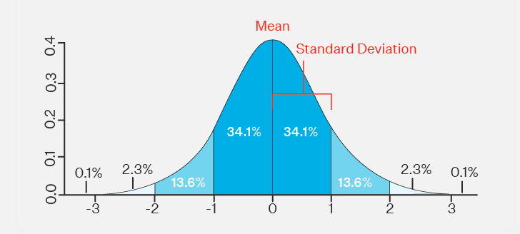
How to calculate std:
It is calculated as the square root of the variance. Variance is the average of the squared differences between the data points and the mean.


|
population standard deviation |
|---|---|

|
the size of the population |

|
each value from the population |

|
the population mean |
Ref: Wikipedia
How do we understand from the data that we need to apply linear regression?
There are a few ways you can understand from the data that linear regression might be an appropriate model to use:
- Linear relationship: If you plot the independent and dependent variables and observe a linear pattern, it suggests that a linear model might be appropriate. You can use a scatterplot to visualize this relationship.
- Correlation: If the independent and dependent variables are correlated, it suggests that a linear model might be appropriate. You can use a correlation coefficient (such as Pearson's r) to measure the strength and direction of the correlation.
- Data type: If the dependent variable is continuous and the independent variables are either continuous or categorical, linear regression might be appropriate. If the dependent variable is categorical, you might want to consider using logistic regression instead.
- Problem type: If you are trying to predict a continuous variable based on other variables, linear regression might be appropriate. If you are trying to classify data into different categories, you might want to consider using a different model such as logistic regression or a decision tree.
How to evaluate a linear regression model?
There are a number of ways to evaluate a linear regression model to assess its performance and understand its strengths and limitations. Here are a few common evaluation metrics:
- R-squared (R^2): This is a measure of how well the model fits the data. It ranges from 0 to 1, with a higher value indicating a better fit. R^2 is calculated as 1 - (SSR/SST), where SSR is the sum of squared residuals (the difference between the predicted and actual values) and SST is the total sum of squares (the difference between the actual values and the mean of the dependent variable).
- Mean squared error (MSE): This is a measure of the average squared difference between the predicted and actual values. A lower MSE indicates a better fit.
- Mean absolute error (MAE): This is a measure of the average absolute difference between the predicted and actual values. A lower MAE indicates a better fit.
- Root mean squared error (RMSE): This is the square root of the MSE and is interpreted in the same units as the dependent variable. A lower RMSE indicates a better fit.
- F-statistic: This is a measure of the overall significance of the model. A high F-statistic indicates that the model is significantly better than a model with no predictors (i.e., a horizontal line).
Why Logistic Regression algorithm named as regression even though it's used for classification
The name "logistic regression" is used because the model is an extension of linear regression, which is used to predict a continuous outcome. However, logistic regression is used for classification, not regression. The model is called "logistic" because it uses the logistic function as the activation function for the model. The logistic function is used to predict the probability that an example belongs to a certain class. The output of the logistic function is always between 0 and 1, which can be interpreted as the probability that the example belongs to the positive class.
The logistic function, also known as the sigmoid function, is a mathematical function that maps any input to a value between 0 and 1. It is defined as follows:
$$ f(x) = \frac{1}{1 + e^{-x}} $$
where e is the base of the natural logarithm, approximately 2.718.
The logistic function has a "S" shape. The output of the function is always between 0 and 1, which makes it convenient for predicting probabilities.
The logistic function is often used as the activation function in neural networks and in logistic regression. In logistic regression, the output of the logistic function is interpreted as the probability that an example belongs to the positive class. The class that the example is assigned to is determined by thresholding the output of the logistic function. For example, if the output is greater than 0.5, the example is classified as the positive class, and if the output is less than 0.5, the example is classified as the negative class.
Why do we normalize data in Machine Learning?
Normalizing data in machine learning is the process of scaling the data so that it has a mean of zero and a standard deviation of one. This is typically done to improve the performance of the machine learning model, by ensuring that the data is in a standardized range and allowing the model to learn more effectively.
For machine learning, every dataset does not require normalization. It is required only when features have different ranges.
For example, consider a data set containing two features, age(x1), and income(x2). Where age ranges from 0–100, while income ranges from 0–20,000 and higher. Income is about 1,000 times larger than age and ranges from 20,000–500,000. So, these two features are in very different ranges. When we do further analysis, like multivariate linear regression, for example, the attributed income will intrinsically influence the result more due to its larger value. But this doesn’t necessarily mean it is more important as a predictor.
Because different features do not have similar ranges of values and hence gradients may end up taking a long time and can oscillate back and forth and take a long time before it can finally find its way to the global/local minimum. To overcome the model learning problem, we normalize the data. We make sure that the different features take on similar ranges of values so that gradient descents can converge more quickly.
In which cases, we don't need to normalize the data?
It is generally a good idea to normalize your data when working with machine learning algorithms. Normalization can help improve the performance of some algorithms, and can also make it easier to compare different data sets. However, there may be some cases where normalization is not necessary. For example, if you are working with algorithms that are not sensitive to the scale of the data, or if the data is already in a normalized format, then normalization may not be necessary. Additionally, if you are working with data that has a natural ordinal relationship, such as grades or rankings, then normalization may not be necessary. It is always a good idea to evaluate your specific use case and data to determine if normalization is necessary.
There are several algorithms that are not sensitive to the scale of the data, and therefore may not require data normalization. Some examples of these algorithms include decision trees, random forests, and support vector machines with linear kernels. These algorithms are not sensitive to the scale of the data because they do not rely on distance measures to make predictions. In these cases, normalization may not be necessary, and could even be detrimental if it distorts the natural relationship between the features in the data. Again, it is always a good idea to evaluate your specific use case and data to determine if normalization is necessary.
What's the difference between data normalization and standardization?
Data normalization and data standardization are two techniques that are often used to pre-process data before it is used in machine learning algorithms. Both techniques are useful for transforming the data in a way that can improve the performance of the algorithms, but they are used for different purposes.
Data normalization is a technique that is used to scale the data so that it is within a specific range, such as 0 to 1. This is done by subtracting the minimum value from each data point and then dividing by the range of the data (the maximum value minus the minimum value). This transformation can help improve the performance of some machine learning algorithms, particularly those that use distance measures, because it ensures that all of the data is on the same scale.
Data standardization, on the other hand, is a technique that is used to transform the data so that it has a mean of 0 and a standard deviation of 1. This is done by subtracting the mean from each data point and then dividing by the standard deviation. This transformation can also help improve the performance of some machine learning algorithms, particularly those that are sensitive to the scale of the data.
When to use data normalization and when to use data standardization?
As a general rule, data normalization is a good technique to use when you want to scale the data to a specific range, such as 0 to 1. This can be useful for algorithms that are sensitive to the scale of the data, such as algorithms that use distance measures. Data standardization, on the other hand, is a good technique to use when you want to transform the data so that it has a mean of 0 and a standard deviation of 1. This can be useful for algorithms that are sensitive to the distribution of the data, such as algorithms that assume that the data is normally distributed.
Normalization -> Data distribution is not Gaussian (bell curve). Typically applies in KNN, ANN
Standardization -> Data distribution is Gaussian (bell curve). Typically applies in Linear regression, logistic regression.
Note: Algorithms like Random Forest (any tree based algorithm) does not require feature scaling.
What are some dimensionality reduction algorithms?
Dimensionality reduction is a technique used to reduce the number of features in a data set, while retaining as much of the relevant information as possible. There are many different algorithms that can be used for dimensionality reduction, and the appropriate algorithm to use will depend on the specific characteristics of the data and the goals of the analysis. Some of the most common dimensionality reduction algorithms include:
- Principal Component Analysis (PCA): PCA is a linear dimensionality reduction algorithm that projects the data onto a lower-dimensional space by maximizing the variance of the data along the principal components. This can be useful for reducing the number of features in the data while retaining as much of the original information as possible.
- Singular Value Decomposition (SVD): SVD is a matrix factorization technique that can be used for dimensionality reduction. It decomposes the data matrix into three matrices, which can then be used to project the data onto a lower-dimensional space.
- Linear Discriminant Analysis (LDA): LDA is a supervised dimensionality reduction algorithm that projects the data onto a lower-dimensional space by maximizing the separation between different classes in the data. This can be useful for improving the performance of classification algorithms.
- t-distributed Stochastic Neighbor Embedding (t-SNE): t-SNE is a non-linear dimensionality reduction algorithm that projects the data onto a lower-dimensional space by preserving the local structure of the data. This can be useful for visualizing high-dimensional data and for uncovering patterns in the data.
Explain Confusion Matrix
A confusion matrix is a table that is often used to describe the performance of a classification algorithm. It provides a detailed breakdown of the correct and incorrect predictions made by the algorithm, allowing you to see how well the algorithm is performing and where it might be making mistakes.
A confusion matrix has four main elements: true positives, true negatives, false positives, and false negatives. True positives are the number of correct predictions that the algorithm made for the positive class. True negatives are the number of correct predictions that the algorithm made for the negative class. False positives are the number of incorrect predictions that the algorithm made for the positive class (i.e. it predicted that the sample was positive, but it was actually negative). False negatives are the number of incorrect predictions that the algorithm made for the negative class (i.e. it predicted that the sample was negative, but it was actually positive).
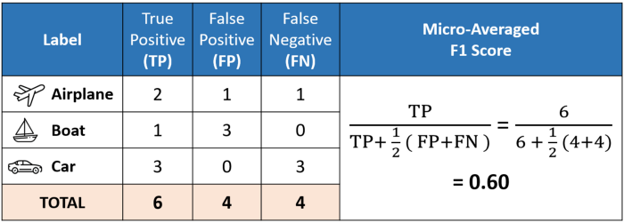
Different evaluation metric calculation
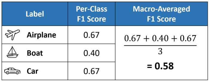
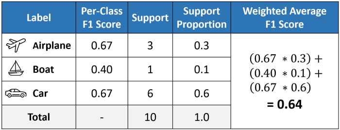
Difference among micro, macro, weighted f1-score
Excellent explanation: medium
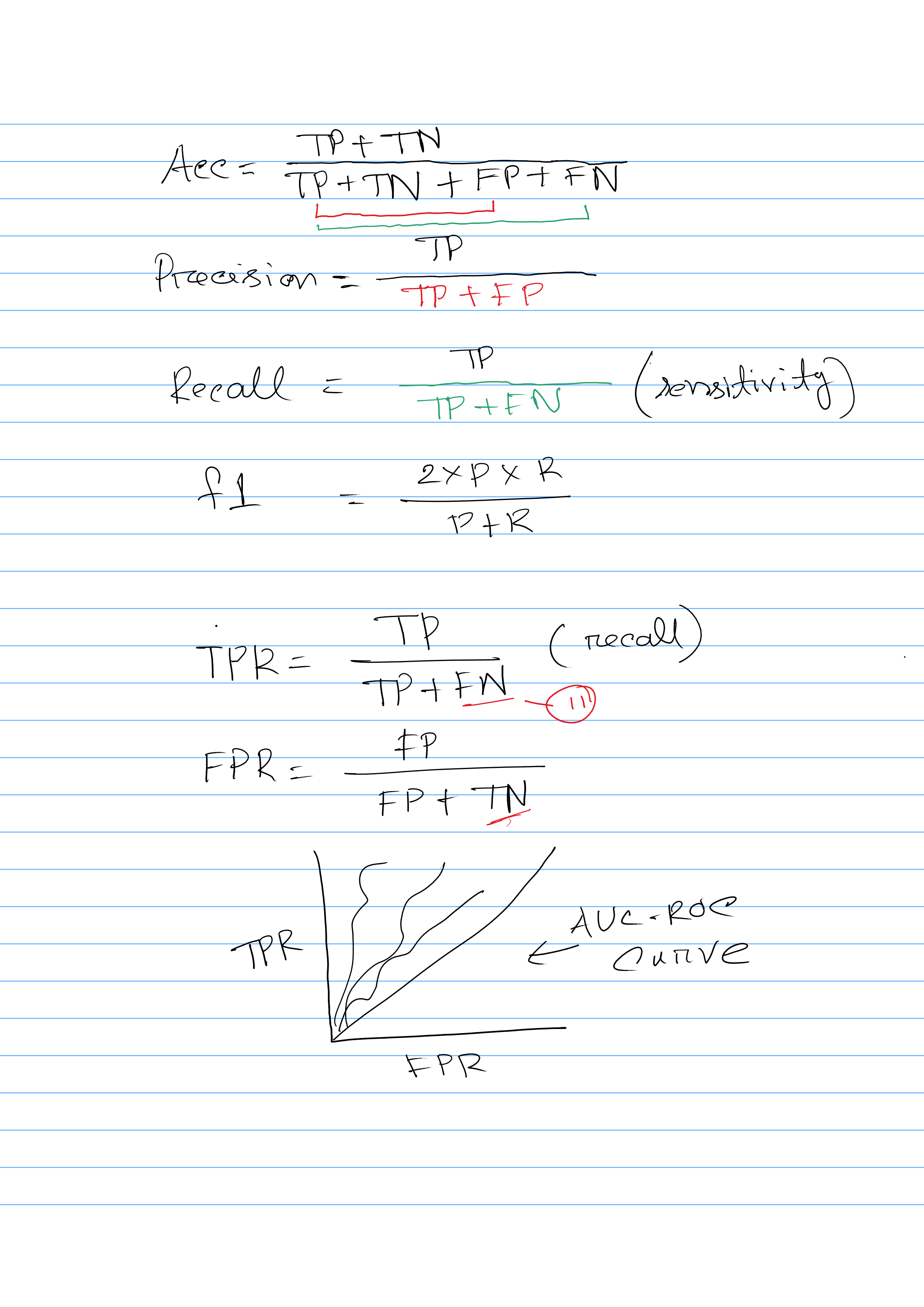
When to use Precision vs Recall vs f1-score
F1-score
When deciding which metric to use, you need to consider the specific goals of your analysis and the potential consequences of false positive and false negative predictions. If you want to minimize false positives, then you should use precision as a metric. If you want to minimize false negatives, then you should use recall as a metric. If avoiding both false positives and false negatives are equally important, then you should use the f1 score as a metric, which is the harmonic mean of precision and recall.
Precision
In some cases, it may be more important to avoid false positives than false negatives. For example, if you are building an AI system to identify criminals in a housing society, then you want to avoid arresting innocent people (false positives), because this could lead to injustice. In this case, you should optimize your model using precision as a metric.
Recall
In other cases, it may be more important to avoid false negatives than false positives. For example, if you are building a security system to screen people for weapons at an airport, then you want to avoid letting dangerous people onto the plane (false negatives), because this could compromise the safety of passengers. In this case, you should optimize your model using recall as a metric.
When to use F1 as a evaluation metric?
The F1 score is a metric that is commonly used to evaluate the performance of a classification model. It is the harmonic mean of the model's precision and recall, which are both calculated by taking the number of true positive predictions by the model and dividing it by the total number of positive predictions made by the model. This means that the F1 score takes into account both the number of false positives and false negatives that the model produces.
One advantage of using the F1 score is that it is a balanced metric, which means that it considers both precision and recall equally. This is useful when you want to avoid a model that has a high precision but low recall, or vice versa. For example, in a medical diagnosis scenario, a model with high precision but low recall may not be useful because it may miss many cases of the disease that it is trying to detect.
When to use AUC-ROC as an evaluation metric?
The AUC-ROC (area under the receiver operating characteristic curve) is a metric that is commonly used to evaluate the performance of a binary classification model. It measures the ability of the model to distinguish between the positive and negative classes.
One advantage of using the AUC-ROC metric is that it is independent of the classification threshold, which means that it is not affected by changes in the threshold used to make predictions. This is useful when you want to compare the performance of different models on the same dataset, or when you want to compare the performance of the same model on different datasets.
Another advantage of the AUC-ROC metric is that it is not sensitive to class imbalance, which means that it can be used when there are unequal numbers of positive and negative instances in the dataset. This is useful when you are working with datasets that have imbalanced classes.
What are the differences between Random Forest and Gradient Boosting?
Random Forest and Gradient Boosting are two popular ensemble learning methods that are used for supervised learning tasks, such as classification and regression. Both methods use multiple decision trees to make predictions, but they differ in the way that the trees are trained and combined.
One key difference between Random Forest and Gradient Boosting is the way that the trees are trained. In Random Forest, the trees are trained independently using a random subsample of the training data. In contrast, in Gradient Boosting, the trees are trained sequentially, with each tree trying to correct the mistakes of the previous tree. This means that the trees in a Gradient Boosting model are more correlated than the trees in a Random Forest model.
Another key difference is the way that the trees are combined to make predictions. In Random Forest, the predictions of all the trees are combined using a majority vote. This means that the final prediction is the class that is predicted by the majority of the trees. In contrast, in Gradient Boosting, the predictions of the trees are combined using a weighted average, where the weights are determined by the performance of each tree.
In general, Random Forest is a good choice for tasks where the goal is to build a robust and accurate model with a low degree of overfitting. It is also a good choice when you have a large number of features in your dataset. In contrast, Gradient Boosting is a good choice for tasks where the goal is to build a highly accurate model, even at the cost of some overfitting.
What's the difference between loss function and cost function?
In machine learning, a loss function and a cost function are similar but distinct concepts. A loss function is a measure of how well a model is able to predict the true values of the target variable given the input data. It quantifies the error between the predicted values and the true values, and is used to guide the training of the model.
In contrast, a cost function is a measure of how well the model is able to make predictions on new data, given the training data. It is a function of the model's parameters, and is used to evaluate the performance of the model.
In other words, a loss function is used to measure the performance of a model on a given training dataset, while a cost function is used to evaluate the performance of the model on unseen data. The loss function is used to update the model's parameters during training, while the cost function is used to compare the performance of different models or the same model with different parameter settings.
In summary,
- The loss function is to capture the difference between the actual and predicted values for a single record
- Whereas cost functions aggregate the difference for the entire training dataset. To do this it aggregates the loss values that are calculated per observation.
A loss function is a part of a cost function.
How do you evaluate the performance of a machine learning model?
There are several ways to evaluate the performance of a machine learning model, including:
- Measuring the model's accuracy: This involves calculating the proportion of correct predictions made by the model on a test dataset. This is a good measure of performance for classification problems, but can be less reliable for regression problems.
- Calculating the model's error: This involves calculating the difference between the predicted values and the true values on the test dataset. This can be done using metrics such as the mean squared error (MSE) for regression problems, or the cross-entropy loss for classification problems.
- Using metrics specific to the type of problem: For example, in a classification problem, metrics such as precision, recall, and F1 score can be used to evaluate the model's performance. In a clustering problem, metrics such as the silhouette score or the Calinski-Harabasz index can be used to evaluate the model's performance.
- Visualizing the model's predictions: This involves creating plots such as scatter plots or histograms to compare the predicted values and the true values. This can help identify patterns and trends in the data and assess the model's performance.
Overall, the choice of evaluation metrics will depend on the specific problem and the goals of the model. It is important to select evaluation metrics that are appropriate for the task and that align with the model's intended use.
Can you describe the concept of regularization and how it can be used to prevent overfitting?
Regularization is a technique used in machine learning to prevent overfitting by adding a penalty term to the loss function of a model. This penalty term, called the regularization term, is typically added to the loss function in the form of a weighted sum of the model's parameters, where the weights are chosen such that large parameter values are penalized more heavily than small ones. This serves to reduce the complexity of the model, which in turn helps to prevent overfitting by limiting the ability of the model to fit the noise in the training data. There are several different types of regularization that can be used, including L1 regularization, L2 regularization, and elastic net regularization.
What is the difference between L1 regularization and L2 regularization
L1 regularization is a technique used in machine learning to prevent overfitting by adding a regularization term to the loss function of a model. The regularization term is the sum of the absolute values of the model's parameters, multiplied by a constant called the regularization parameter. This can be written mathematically as follows:
1L1 regularization term = regularization_parameter * sum(|parameters|)
where regularization_parameter is a hyperparameter that determines the strength of the regularization, and parameters is a vector of the model's parameters.
L2 regularization is another technique used to prevent overfitting by adding a regularization term to the loss function. In L2 regularization, the regularization term is the sum of the squares of the model's parameters, multiplied by a constant called the regularization parameter. This can be written mathematically as follows:
1L2 regularization term = regularization_parameter * sum(parameters^2)
where regularization_parameter is a hyperparameter that determines the strength of the regularization, and parameters is a vector of the model's parameters.
Both L1 and L2 regularization are used to reduce the complexity of a model and prevent overfitting, but they do so in different ways.
-
L1 regularization encourages the model to use only a subset of its features.
-
While L2 regularization discourages the model from using very large parameter values.
How do you handle missing or incorrect data in your data science project?
There are several approaches that can be used to handle missing data in a data science project, depending on the specific needs of the project and the goals of the analysis. Some common approaches include:
-
Removing rows or columns that contain missing data: This approach can be useful if the missing data is not representative of the overall dataset, or if the amount of missing data is relatively small.
-
Imputing the missing data using a statistical method: This approach can be useful if the missing data is not random, and if there is a clear pattern or relationship between the missing data and other values in the dataset.
-
Using data from a different source to fill in the missing data: This approach can be useful if there is another dataset that contains information that is relevant to the missing data, and if it is possible to combine the two datasets in a meaningful way.
-
Ignoring the missing data and proceeding with the analysis using only the available data: This approach can be useful if the amount of missing data is relatively small, and if it is not likely to significantly impact the results of the analysis.
-
If there are outliers in the data, we can replace the missing data with median of the feature.
-
Better way would be to use KNN to find the similar observations/samples, and then replace missing values with their (similar samples) average.
KNN works better for numerical data.
How do you handle large datasets?
- Sampling: This involves selecting a representative subset of the data to work with, rather than using the entire dataset. This can be useful if the dataset is too large to work with efficiently, or if the patterns and trends in the data can be accurately represented by a smaller sample.
- Parallel processing: This involves using multiple computers or processors to perform the analysis simultaneously, rather than using a single processor. This can be useful if the dataset is too large to fit into the memory of a single computer, or if the analysis requires a lot of computational power.
- Data reduction: This involves applying techniques such as feature selection or dimensionality reduction to reduce the number of variables or features in the dataset. This can be useful if the dataset contains a large number of redundant or irrelevant variables, or if the analysis can be performed more efficiently with a smaller number of variables.
- Data partitioning: This involves dividing the dataset into smaller subsets and performing the analysis on each subset separately. This can be useful if the dataset is too large to work with efficiently, or if the analysis can be performed more efficiently in smaller chunks.
How do you stay up-to-date with the latest developments in data science and machine learning?
There are several ways to stay up-to-date with the latest developments in data science and machine learning. Some common approaches include:
- Following notable people on Twitter who are working with AI/ML technologies. They usually share a lot of news about new trends in the industry and academia.
- Reading books and articles on data science and machine learning: This can help you stay current with the latest theories, techniques, and applications in the field.
- Attending conferences and workshops: This can provide you with opportunities to learn from experts in the field, and to network with other professionals working in data science and machine learning.
- Joining online communities and forums: This can provide you with access to a wealth of knowledge and resources, and can also provide opportunities to connect with other data scientists and machine learning professionals.
- Participating in online courses and training programs: This can provide you with structured learning experiences, and can also help you stay up-to-date with the latest tools and technologies in the field.
- Staying current with industry news and trends: This can help you stay informed about the latest developments and innovations in the field, and can also provide valuable insights into how data science and machine learning are being used in the real world.
How dimensionality reduction work in Machine Learning
Dimensionality reduction is a technique that is used in machine learning to reduce the number of features or dimensions in a dataset. This is useful because it can make the data easier to work with and analyze, and can also improve the performance of machine learning algorithms.
There are several ways that dimensionality reduction can be implemented in machine learning, including:
- Feature selection: This involves selecting a subset of the most important features from the dataset, and removing the others. This can be useful if the dataset contains a large number of redundant or irrelevant features, or if the analysis can be performed more efficiently with a smaller number of features.
- Principal component analysis (PCA): This is a statistical technique that uses linear algebra to transform the data into a new space with fewer dimensions, while preserving as much of the original variance in the data as possible. This can be useful if the data is highly correlated, or if there is a strong linear relationship between the features.
- Autoencoders: These are artificial neural networks that are trained to learn a compact representation of the data, by encoding the data into a lower-dimensional space and then decoding it back into the original space. This can be useful if the data is non-linear, or if there is a complex relationship between the features.
How PCA works?
Principal component analysis (PCA) is a statistical technique that is often used for dimensionality reduction in machine learning. It is a method that uses linear algebra to transform the data into a new space with fewer dimensions, while preserving as much of the original variance in the data as possible.
Here is a step-by-step explanation of how PCA works for dimensionality reduction:
- Standardize the data: The first step is to standardize the data by subtracting the mean from each feature and dividing by the standard deviation. This is necessary because PCA is sensitive to the scale of the data, and standardizing the data ensures that all the features are on the same scale.
- Compute the covariance matrix: The next step is to compute the covariance matrix of the standardized data. This is a square matrix that contains the pairwise covariances between all the features in the data.
- Compute the eigenvectors and eigenvalues: The next step is to compute the eigenvectors and eigenvalues of the covariance matrix. The eigenvectors are the directions in the data space along which the data varies the most, and the eigenvalues are the corresponding magnitudes of the variations.
- Select the eigenvectors with the highest eigenvalues: The next step is to select the eigenvectors with the highest eigenvalues, as these are the directions in the data space that capture the most variance.
- Transform the data into the new space: The final step is to transform the data into the new space defined by the selected eigenvectors. This is done by computing the dot product of the standardized data and the eigenvectors, which projects the data onto the new space.
By using PCA for dimensionality reduction, data scientists and machine learning professionals can reduce the complexity of the data, and improve the performance of machine learning algorithms. Additionally, PCA can also be used to visualize high-dimensional data in a lower-dimensional space, which can help to gain insights into the underlying structure of the data.
What are the different types of data distribution in statistics?
In statistics, data can be distributed in many different ways, depending on the characteristics of the data and the underlying population. Some common distributions of data include:
- Normal distribution: This is a symmetrical distribution that is often described as a bell-shaped curve. It is commonly used to model data that is continuous and normally distributed, such as height, weight, or IQ.
- Binomial distribution: This is a distribution that is used to model data that can take on only two possible values, such as success or failure, or heads or tails. It is commonly used to model the probability of a certain number of successes in a given number of trials.
- Poisson distribution: This is a distribution that is used to model data that represents the number of events that occur in a given time or space. It is commonly used to model data that is discrete and counts the number of occurrences of an event, such as the number of accidents on a highway or the number of defects in a manufacturing process.
- Exponential distribution: This is a distribution that is used to model data that is continuous and has a constant rate of change. It is commonly used to model data that represents the time between events, such as the time between arrivals at a bus stop or the time between failures of a machine.
- Uniform distribution: This is a distribution that is used to model data that is continuous and has an equal probability of occurring within a given range. It is commonly used to model data that is randomly generated, such as the results of a dice roll or a random number generator.
What are some clustering algorithm in Machine Learning?
Clustering is a technique that is used to group data points into clusters based on their similarity. This can be useful for a variety of applications, such as image segmentation, customer segmentation, and anomaly detection. Some common clustering algorithms include:
- K-means: This is a popular and widely-used clustering algorithm that is based on the idea of partitioning the data into a specified number of clusters, and then iteratively refining the cluster assignments until the clusters are as compact and well-separated as possible.
- Hierarchical clustering: This is a clustering algorithm that is based on the idea of building a hierarchy of clusters, where each cluster is split into smaller clusters until each data point belongs to a single-point cluster.
- DBSCAN: This is a clustering algorithm that is based on the idea of finding dense clusters of data points in the data space, and then expanding the clusters to include points that are nearby.
- Expectation-maximization (EM): This is a clustering algorithm that is based on the idea of fitting a mixture model to the data, where each component of the mixture represents a different cluster.
What are the different feature selection procedures in Machine Learning?
- Correlation-based Feature Selection: This technique calculates the correlation between each feature and the target variable and only keeps the features with a high correlation. This can be useful for removing redundant features that add little predictive power to the model.
- Wrapper-based Feature Selection: This technique uses a predictive model to evaluate each feature's importance, then selects the features that improve the model's performance. This is a more computationally intensive method, but it can be effective for selecting the most relevant features.
- Embedded-based Feature Selection: This technique trains a predictive model and then uses the model's weights to determine each feature's importance. Features with high absolute weight are important and retained in the model. This is a good method for selecting useful features for making predictions.
- Recursive Feature Elimination (RFE): This technique recursively removes features, builds a model using the remaining features, and then evaluates the model's performance. The process is repeated until only the most relevant features are left.
- Principal Component Analysis (PCA): This technique projects the data onto a lower-dimensional space and selects the most important principal components for building the model. This can be useful for reducing the dimensionality of the data and removing irrelevant features.
In general, the best approach for feature selection will depend on the specific dataset and the type of model being used. It is important to experiment with different methods to find the one that works best for your particular situation.
How to select features for a xgboost model?
To select features for a xgboost model, you can use the SelectFromModel method, which is part of the scikit-learn library. This method allows you to specify a threshold for feature importance, and then automatically selects the features that meet or exceed that threshold.
 1import xgboost as xgb
 2from sklearn.feature_selection import SelectFromModel
 3
 4# Train your xgboost model
 5model = xgb.XGBClassifier()
 6model.fit(X_train, y_train)
 7
 8# Use SelectFromModel to select features with a minimum importance value of 0.2
 9selection = SelectFromModel(model, threshold=0.2)
10selected_features = selection.transform(X_train)
11
12# Train a new model using only the selected features
13new_model = xgb.XGBClassifier()
14new_model.fit(selected_features, y_train)
The SelectFromModel method is used to select all of the features that have an importance value of at least 0.2, as determined by the trained xgboost model. These selected features are then used to train a new xgboost model.
You can adjust the threshold value to select more or fewer features, depending on your needs. It's generally a good idea to use a relatively low threshold value, to ensure that you are selecting as many relevant features as possible. However, if your dataset has a large number of features and you want to reduce the number of features for computational efficiency, you can use a higher threshold value to select only the most important features.
How Neural Networks work?
Neural networks are a type of machine learning algorithm that are inspired by the structure and function of the human brain. They are composed of many interconnected processing units, called neurons, that are arranged into layers. The neurons in the input layer receive input data, and the neurons in the output layer produce the final output of the network. The neurons in the hidden layers process the data and pass it on to the next layer.
Step-by-step explanation of how a neural network works:
Initialize the weights: The first step is to initialize the weights of the connections between the neurons in the network. The weights are typically initialized to small random values, in order to break any symmetry in the network and allow the network to learn from the data.
Feed the input data through the network: The next step is to feed the input data through the network, by passing the data from the input layer to the first hidden layer. At each layer, the neurons compute a weighted sum of the inputs, and then apply an activation function to the sum in order to produce an output.
Propagate the output through the network: The next step is to propagate the output of each layer through the network, by passing the output from one layer to the next. This continues until the output of the final layer is produced, which represents the final output of the network.
Calculate the error: The next step is to calculate the error between the actual output of the network and the desired output. This error is used to measure the performance of the network and to guide the learning process.
Adjust the weights: The final step is to adjust the weights of the connections between the neurons in the network in order to reduce the error. This is typically done using a gradient descent algorithm, which computes the gradient of the error with respect to the weights and updates the weights in the direction that reduces the error.
By repeating these steps, the neural network can learn from the data and improve its performance over time. As the network learns, the weights of the connections between the neurons are adjusted in order to capture the underlying patterns and relationships in the data. This allows the network to make accurate predictions and decisions based on the input data.
How the Backpropagation algorithm works
Backpropagation is an algorithm used to train neural networks. It is used to compute the gradients of the loss function with respect to the weights of the network, so that the weights can be updated to minimize the loss.
The process of backpropagation can be broken down into the following steps:
Forward propagation: During forward propagation, the inputs are passed through the network and the predictions are made. The prediction error is then calculated using the loss function.
Backward propagation: During backward propagation, the error is backpropagated through the network, starting at the output layer and working backwards layer by layer. The error at each layer is used to calculate the gradients of the loss function with respect to the weights of the network.
Weight update: Once the gradients of the loss function with respect to the weights have been calculated, the weights can be updated using an optimization algorithm, such as stochastic gradient descent (SGD).
Repeat: The process of forward propagation, backward propagation, and weight update is repeated until the loss function is minimized.
Backpropagation is an efficient way to calculate the gradients of the loss function with respect to the weights of the network, which makes it an important algorithm in the training of neural networks.
What is Gradient Descent, and what are the different versions of Gradient Descent
Gradient descent is an optimization algorithm that is used to minimize a loss function. It works by adjusting the parameters of a model in small increments to minimize the loss.
Imagine you are at the top of a mountain and you want to find the path that leads to the bottom of the mountain. The bottom of the mountain represents the minimum of the loss function, and the parameters of the model are like your position on the mountain. The gradient of the loss function with respect to the parameters is like the slope of the mountain at your position. To find the minimum of the loss function, you can follow the direction of the gradient downhill until you reach the bottom of the mountain.
This is an oversimplification, but it gives the basic idea of how gradient descent works. In practice, the algorithm starts with an initial set of parameter values and then iteratively adjusts the values in the direction that reduces the loss. The magnitude of the update to the parameters is determined by the learning rate. The process is repeated until the loss function is minimized or a maximum number of iterations is reached.
Gradient descent is a widely used optimization algorithm in machine learning and is commonly used to train neural networks. There are several variations of gradient descent, such as batch gradient descent, stochastic gradient descent, and mini-batch gradient descent, which are used in different situations.
Batch gradient descent: In batch gradient descent, the gradient is calculated for the entire training set and the parameters are updated all at once. This can be computationally expensive when the training set is large, but it is generally the most accurate method.
Stochastic gradient descent: In stochastic gradient descent, the gradient is calculated for each training example and the parameters are updated after each example. This can be faster than batch gradient descent because the update is performed after each example, but it can also be less stable because the updates are based on a single example.
Mini-batch gradient descent: In mini-batch gradient descent, the gradient is calculated for a small batch of training examples and the parameters are updated after each batch. This can be faster than batch gradient descent because the update is performed after a small number of examples, but it can also be less stable because the updates are based on a small number of examples.
Accelerated gradient descent: There are several variants of gradient descent that use techniques such as momentum and Nesterov acceleration to improve the convergence rate of the algorithm. These techniques can help the algorithm escape from local minima and converge to the global minimum more quickly.
Which version of gradient descent to use depends on the problem at hand and the available computational resources. In general, mini-batch gradient descent is a good compromise between the speed of stochastic gradient descent and the stability of batch gradient descent.
Explain different different types of layers in a Neural Network
Fully Connected Layers: These are like a basic building block of a neural network that helps it learn patterns in the data. Each neuron in a layer is connected to every neuron in next layer, allowing the network to learn complex relationships between the inputs and outputs.
Convolutional Layers: These layers are used in image and video recognition tasks. They help the network to recognize patterns in the image, such as edges, shapes, or textures, by applying a filter to the image and looking for specific features.
Pooling Layers: These layers are used to reduce the size of the image or feature map that comes out of a convolutional layer. Max pooling is a common type of pooling layer that takes the maximum value of a set of values in the feature map.
Recurrent Layers: These layers are used to process sequential data, such as text or time-series data. They allow the network to remember information from previous time steps, which can be helpful in predicting the next value in a sequence.
Normalization Layers: These layers are used to normalize the output of the previous layer to improve the stability and performance of the network. They make sure that the data going into the next layer is on the same scale and is easier to process.
Dropout Layers: These layers are used to prevent overfitting, which happens when the network becomes too specialized to the training data and doesn't generalize well to new data. Dropout randomly drops out some of the neurons in a layer during training, which makes the network more robust to noise and variation in the data.
Embedding Layers: These layers are used to represent categorical data, such as words or user IDs, as continuous vectors that can be fed into the neural network. This makes it easier for the network to process and learn patterns in the data.
Activation Layers: These layers apply a nonlinear function to the output of the previous layer, introducing nonlinearity into the model. This allows the network to learn complex relationships between the inputs and outputs that wouldn't be possible with a linear model.
Self-Attention Layers: These layers are commonly used in transformer-based models such as BERT or GPT-3. They allow the model to attend to different parts of the input sequence when processing each token.
Skip-Connection Layers: These layers allow the network to skip over one or more layers during training. This can help to prevent the vanishing gradient problem and improve the performance of the network.
Spatial Transformer Layers: These layers allow the network to learn to transform the input data in a spatially-varying way. This can be useful in tasks such as image segmentation, where the network needs to learn to focus on different parts of the image.
Residual Layers: These layers are used in residual networks (ResNets) to allow the network to learn residual functions. This can help to prevent the vanishing gradient problem and improve the performance of the network.
Capsule Layers: These layers are used in capsule networks to allow the network to learn structured representations of objects. This can be useful in tasks such as object recognition or pose estimation.
What are the building blocks of a Convolutional Neural Networks (CNNs)
Convolutional neural networks (CNNs) are a type of neural network that is specifically designed to work with data that has a grid-like structure, such as an image. CNNs are comp0sed of multiple layers of interconnected neurons, where the neurons in each layer are arranged in a three-dimensional grid. The building blocks of a CNN include:
Input layer: The input layer receivess the input data and passes it on to the first hidden layer. In the case of an image, the input layer consists of multiple neurons, each representing a pixel in the image.
Hidden layers: The hidden layers are composed of multiple neurons arranged in a three-dimensional grid. Each neuron in a hidden layer receives inputs from a small region of the previous layer, and produces an output that is passed on to the next layer.
Convolutional layers: In a CNN, the hidden layers typically include convolutional layers, where the neurons perform a convolution operation on the input data. This involves applying a small kernel or filter to the input data, which extracts features from the data and passes them on to the next layer.
Pooling layers: The hidden layers of a CNN may also include pooling layers, where the neurons perform a down-sampling operation on the input data. This involves summarizing the input data in some way, such as taking the maximum or average value, in order to reduce the dimensionality of the data and make the network more robust to changes in the input data.
Fully-connected layers: The final hidden layers of a CNN are typically fully-connected, where each neuron receives inputs from all the neurons in the previous layer. This allows the network to combine the extracted features from the convolutional and pooling layers, and make a prediction or decision based on the input data.
**Batch Normalization layers **: Batch Normalization is a technique for training deep neural networks that standardizes the inputs to a layer for each mini-batch. It has the effect of stabilizing the learning process and dramatically reducing the number of epochs required to train a deep learning model. Batch normalization works by normalizing the activations of a layer for each mini-batch. This has the effect of making the distribution of the activations more stable, which in turn makes it easier to train the model. It also has the effect of regularizing the model, which can reduce overfitting.
Output layer: The output layer produces the final output of the network. In the case of an image classification task, the output layer may consist of multiple neurons, each representing a different class. The output of the network is the predicted class of the input image.
Explain Stride in CNN
In a Convolutional Neural Network (CNN), the stride is the number of pixels that the convolutional filter moves each time it is applied to the input. The stride is a hyperparameter of the CNN, and it can be adjusted to control the size of the output produced by the convolutional layer.
For example, consider a CNN with an input of size 32x32 and a convolutional layer with a kernel size of 3 and a stride of 2. This means that the convolutional filter will be applied to the input in a sliding window fashion, moving 2 pixels at a time. The output of this convolutional layer will be 16x16, since the filter is applied to every other pixel in the input.
Increasing the stride can reduce the size of the output produced by the convolutional layer, which can help to reduce the number of parameters in the model and improve the training process. However, it can also reduce the amount of information that is captured by the convolutional layer, which can degrade the performance of the model.
How to calculate the number of parameters and output shape size for CNN?
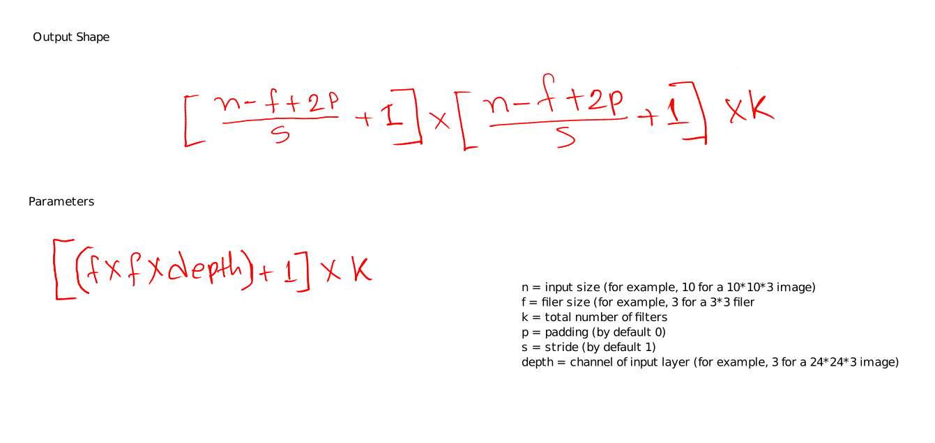
What are some of the state-of-the-art Computer Vision models
- ResNet: This is a deep convolutional neural network that is trained on large datasets and is capable of achieving high accuracy on many tasks.
- DenseNet: This is another deep convolutional neural network that is known for its ability to efficiently learn complex representations.
- Inception: This is a model that uses a combination of convolutional and pooling layers to learn features from images.
- Mask R-CNN: This is a model that is specifically designed for object detection and instance segmentation, which involves identifying and segmenting individual objects in an image.
- GANs: Generative adversarial networks are a class of models that can be used to generate new images based on a given input.
- YOLO (You Only Look Once): This is a fast object detection model that can be used to identify objects in real-time.
- R-CNN (Regional Convolutional Neural Network): This is a model that uses region proposal algorithms to identify objects in an image and then uses a CNN to classify the objects.
- SSD (Single Shot Detector): This is a model that combines a CNN with a regression layer to identify objects in an image.
- U-Net: This is a model that is specifically designed for image segmentation, which involves dividing an image into multiple segments or regions.
- VGG (Visual Geometry Group): This is a model that uses a series of convolutional and pooling layers to learn features from images.
How a Recurrent Neural Network (RNN) works
An RNN is a type of neural network that is designed to process sequential data. It does this by using a "memory" that allows it to remember important information from the past, which it can use to inform its processing of the current input.
The basic building block of an RNN is the "recurrent neuron," which has a single input and a single output, but it also has a "memory" in the form of a hidden state. The hidden state is a vector of values that is maintained by the neuron and is used to store information from the past.
At each time step, the recurrent neuron receives an input and combines it with its current hidden state to produce an output and a new hidden state. The output and the new hidden state are then used as input for the next time step. This allows the RNN to maintain a "memory" of the input data and use it to inform its processing of the current input.
RNNs can have many layers, and each layer consists of a set of recurrent neurons. The input data is passed through the layers of the RNN in a sequential manner, with the output of each time step being used as input for the next time step. This allows the RNN to capture patterns and dependencies over longer time periods.
RNNs are trained using a variant of gradient descent, such as mini-batch gradient descent or stochastic gradient descent. During training, the weights of the recurrent neurons are adjusted to minimize the error between the predicted output and the ground truth.
RNNs are widely used in natural language processing tasks, such as language translation, language generation, and text classification.
There are several types of RNNs, including:
- Simple RNNs: These are the simplest type of RNN, and they have a single hidden layer that processes the input data sequentially.
- Long Short-Term Memory (LSTM) Networks: These are a more advanced type of RNN that have additional gates that control the flow of information through the network. LSTMs are particularly useful for tasks that require the network to remember information over long periods of time.
- Gated Recurrent Units (GRUs): These are another type of advanced RNN that have a similar structure to LSTMs, but they have fewer parameters and are easier to train.
Main difference between LSTM and GRU
Long Short-Term Memory (LSTM) networks and Gated Recurrent Units (GRUs) are both types of Recurrent Neural Networks (RNNs) that are designed to process sequential data. They both have a "memory" that allows them to remember important information from the past, which they can use to inform their processing of the current input.
The main difference between LSTMs and GRUs is the way they maintain their "memory." LSTMs have three different types of gates that control the flow of information through the network: the input gate, the output gate, and the forget gate. These gates allow LSTMs to selectively choose which information to remember and which to forget, which makes them very effective at learning long-term dependencies.
GRUs, on the other hand, have a single update gate that controls the flow of information through the network. The update gate determines which information to retain from the previous hidden state and which to discard. GRUs are simpler than LSTMs and have fewer parameters, which makes them easier to train.
Both LSTMs and GRUs have been successful at a wide range of natural language processing tasks, such as language translation, language generation, and text classification. However, LSTMs tend to be more powerful and are generally considered to be the better choice for tasks that require the network to remember information over long periods of time. GRUs are a good choice when you want a simpler and faster model that is still able to capture long-term dependencies.
What is the difference between batch prediction and online prediction?
Batch prediction and online prediction are two different methods for making predictions using machine learning models.
Batch prediction involves using a trained machine learning model to make predictions on a large batch of data all at once. This is typically done by feeding the entire dataset into the model, and then using the model to make predictions on each data point in the batch. Batch prediction is useful when the dataset is large and the predictions can be made in parallel, as it can be more efficient than making predictions one at a time.
Online prediction involves using a trained machine learning model to make predictions on individual data points as they are received. This is useful when the data is streaming or the predictions need to be made in real-time, as it allows the model to make predictions on the fly.
Give a real-life example of when to use batch inference and when to use online inference
Batch inference is typically used when you have a large amount of data that you need to process all at once, such as when you are running a machine learning model on a dataset to make predictions. Online inference, on the other hand, is used when you need to make predictions on individual data points in real-time, such as when you are using a speech-to-text model to transcribe audio in real-time.
For example, if you are building a system to classify images, you might use batch inference to process a dataset of images and train a machine learning model. Once the model is trained, you could then use online inference to classify new images as they come in, in real-time.
Another example might be a website that uses a machine learning model to recommend products to customers. In this case, you could use batch inference to process the entire catalog of products and train a recommendation model, and then use online inference to generate personalized recommendations for individual users as they browse the website.
How to reduce the prediction serving latency in Machine Learning?
There are a few different ways to reduce the prediction serving latency in machine learning, including the following:
- Optimize the model for inference: One way to reduce the prediction serving latency is to optimize the model for inference. This can involve techniques such as quantizing the model to reduce the number of bits used to represent the weights, or pruning the model to remove redundant or unnecessary connections.
- Use a faster hardware platform: Another way to reduce the prediction serving latency is to use a faster hardware platform for serving the model. For example, you could use a high-performance GPU or a custom ASIC designed for machine learning inference to speed up the processing of predictions.
- Use a faster inference algorithm: Some machine learning models can be served using different inference algorithms, which can have different performance characteristics. Choosing a faster inference algorithm can help reduce the prediction serving latency.
- Use a cache: If your model is serving a large number of requests, it can be helpful to use a cache to store the results of previous predictions. This can allow you to quickly serve the same request multiple times without having to re-run the entire model.
- Use a distributed serving architecture: Finally, using a distributed serving architecture can also help reduce the prediction serving latency. This involves running multiple instances of the model on different machines, and using a load balancer to distribute incoming requests across the different instances. This can help reduce the time it takes to serve each individual request.
Explain how pre-trained BERT embeddings are generated.
Pretrained BERT embeddings are generated by training a BERT model on a large corpus of text data. The BERT model is a type of Transformer-based neural network that is designed to process and understand natural language. During training, the model learns to generate a numerical representation, or embedding, for each word in the training corpus. These word embeddings capture the semantic meaning of the words and can be used as input to other natural language processing models.
How do the pre-trained weights understand completely new unseen word representation?
Pretrained BERT models are not specifically designed to understand completely new words that they have not seen during training. Instead, they rely on a process called subword tokenization, which breaks words down into smaller pieces called subwords. For example, the word "unexpected" might be broken down into the subwords "un", "expect", and "ed". The BERT model can then generate an embedding for each subword, which can be combined to represent the overall meaning of the original word. This allows the model to generalize to words that it has not seen in the training data, by using the subwords that it has learned to represent similar words.
What's the workflow of a text summarization in NLP using pre-trained weights?
The workflow of a text summarization model using pretrained weights would generally involve the following steps:
- Preprocessing the input text data to clean and prepare it for input to the model. This may involve tokenizing the text, removing punctuation and stop words, and extracting important keywords and phrases.
- Loading the pretrained weights into the model, which would have been trained on a large corpus of text data.
- Feeding the preprocessed input text into the model, which would generate a numerical representation, or embedding, for each word in the text.
- Using the word embeddings as input to the summarization model, which would generate a summary of the input text. This summary may be a shorter version of the original text, or it may highlight the most important points in the text.
- Postprocessing the output summary to clean and format it, and outputting it in the desired format.
This is a general outline of the process, and specific implementations may vary depending on the details of the model and the data.
What are the different approaches to generating word embeddings in NLP?
- Word2Vec: This is a popular method for learning word embeddings by predicting the surrounding words in a sentence or phrase.
- GloVe: This method learns word embeddings by training a model to predict the co-occurrence of words in a corpus of text data.
- FastText: This method learns word embeddings by training a model to predict the words in a sentence, based on the characters in the words.
- BERT: This method uses a transformer-based neural network to learn word embeddings by training on a large corpus of text data.
How to generate embeddings for a Computer Vision task?
To generate embeddings for a computer vision task, you would typically use a convolutional neural network (CNN) to extract features from the input images. The CNN would be trained on a large dataset of images, and during training, it would learn to generate a numerical representation, or embedding, for each image. This embedding would capture the key features of the image, and could be used as input to other machine learning models for tasks such as image classification or object detection.
To generate the embeddings, you would first preprocess the input images by resizing them to a fixed size and converting them to a format that is suitable for input to the CNN. You would then feed the preprocessed images into the CNN, which would generate the embeddings. These embeddings could then be used as input to other machine learning models for downstream tasks.
What's the difference between the BERT model and the SBERT model?
BERT, or Bidirectional Encoder Representations from Transformers, is a type of transformer-based neural network that is designed to process and understand natural language. SBERT, or Sentence-BERT, is a variation of BERT that is specifically designed to encode sentences rather than individual words. This allows SBERT to capture the meaning of entire sentences, rather than just the individual words, which can be useful for certain natural language processing tasks such as sentiment analysis or text classification.
One key difference between the BERT and SBERT models is the input data that they are designed to process. BERT is typically trained on a large corpus of text data and is designed to generate word embeddings, which capture the semantic meaning of individual words. In contrast, SBERT is trained to generate sentence embeddings, which capture the meaning of entire sentences. This allows SBERT to better capture the context and meaning of sentences, which can be useful for certain natural language processing tasks.
Another key difference between the two models is their performance and accuracy. BERT is a highly accurate model, but it is designed to process individual words, so it may not always capture the meaning of longer phrases or sentences. SBERT, on the other hand, is specifically designed to process entire sentences, so it may be more accurate for tasks that require understanding the meaning of longer phrases or sentences. However, SBERT is a relatively new model, so its performance has not been extensively tested and evaluated.
How a video classification works
There are many different architectures that can be used for video classification tasks, and the best architecture for a particular task will depend on the specific requirements and constraints of the task. Some commonly used architectures for video classification include:
-
CNNs + LSTM: These are particularly well-suited for processing image data, and can be used to extract features from each frame of a video. CNNs can be combined with other types of neural networks, such as long short-term memory (LSTM) networks, to take into account the temporal dependencies between the frames of the video.
-
3D convolutional neural networks (3D CNNs): These are similar to CNNs, but are designed to process data with a temporal dimension, such as video data. They are able to learn spatiotemporal features from the video data by applying convolutional filters to the data in three dimensions (i.e., width, height, and time).
-
Two-stream neural networks: These are a type of architecture that combines the outputs of a CNN that processes the raw video frames with the outputs of a CNN that processes optical flow maps of the video. Optical flow maps capture the motion between frames in a video, and can provide additional information about the motion and dynamics of the objects in the video.
Temporal dependencies refer to the relationships between events or variables that are dependent on the time at which they occur. In the context of a video classifier, temporal dependencies refer to the relationships between the frames of the video and how they change over time.
For example, consider a video of a person walking. Each frame of the video represents a snapshot of the person's appearance at a particular point in time. The temporal dependencies between these frames would include the person's motion and the changes in their appearance as they walk. A model that is able to take into account these temporal dependencies would be able to use information from multiple frames in the video to better understand the person's actions and make a more informed classification decision.
LSTM networks are particularly well-suited for modeling temporal dependencies because they are able to remember information from previous timesteps in a sequence and use this information to inform their decisions at later timesteps. This allows them to effectively model the changing relationships between the frames of a video over time.
CNN+LSTM network
A video classifier that uses a combination of convolutional neural networks (CNNs) and long short-term memory (LSTM) networks can work by taking in a video as input and processing it through the CNN portion of the model to extract features from each frame of the video. These features are then passed to the LSTM portion of the model, which takes into account the sequence of frames in the video and the temporal dependencies between them to make a classification decision.
The CNN portion of the model is responsible for learning features from the individual frames of the video that are relevant for the classification task. This is done using convolutional layers, which apply a set of filters to the input data and learn to recognize patterns and features within the data.
The LSTM portion of the model is a type of recurrent neural network that is designed to process sequential data. It is able to remember information from previous timesteps in the sequence and use this information to inform its classification decision.
Together, the CNN and LSTM portions of the model are able to take into account both the individual frames of the video and the temporal dependencies between them to make a classification decision. This allows the model to learn to recognize complex patterns and behaviors in the video data and make more accurate classification decisions.
3D CNNs
3D convolutional neural networks (3D CNNs) are a type of neural network that is designed to process data with a temporal dimension, such as video data. They are particularly well-suited for tasks such as video classification, action recognition, and anomaly detection.
3D CNNs are similar to traditional convolutional neural networks (CNNs), but are designed to apply convolutional filters to the data in three dimensions (i.e., width, height, and time). This allows them to learn spatiotemporal features from the data, which are features that capture both the spatial relationships between the pixels in an image and the temporal dependencies between the frames in a video.
To apply 3D convolutional filters to the data, 3D CNNs typically use a kernel that is three-dimensional (i.e., a cube) rather than a kernel that is two-dimensional (i.e., a square). This kernel is then moved across the data in all three dimensions (width, height, and time) and convolved with the data to produce a feature map. The process is then repeated using different kernels to learn multiple features from the data.
3D CNNs typically consist of multiple layers of 3D convolutional filters, followed by non-linear activation functions, and may also include pooling layers and fully connected layers. The output of the final layer of the network can be used for tasks such as classification or regression.
3D CNNs are able to learn complex spatiotemporal features from the data and can be trained to recognize patterns and behaviors in the data that are not easily detectable using other approaches. However, they can be computationally intensive to train and may require large amounts of data to achieve good performance.
Why do we use the activation functions?
Activation functions are used in artificial neural networks to introduce non-linearity. Without activation functions, neural networks would be limited to linear models, which are not very powerful. Activation functions allow neural networks to model complex relationships between input and output.
Activation functions also help normalize the output of a neuron so that it falls within a specific range, which can be useful for modeling probability or for creating stable and consistent models.
There are many different activation functions to choose from, and the choice of activation function can have a big impact on the performance of the neural network. Some commonly used activation functions include the sigmoid function, the tanh function, and the ReLU (Rectified Linear Unit) function.
Why ReLU works better than others?
The ReLU (Rectified Linear Unit) activation function has become very popular in recent years because it has been shown to work well in a wide range of deep learning models. The ReLU function is defined as
1f(x) = max(0, x)
where x is the input to the activation function.
There are several reasons why the ReLU function has become so popular:
- It is very simple to compute, requiring only a simple max operation. This makes it very efficient to compute, especially in large models where the activation function is called many times.
- It has been shown to work well in practice. It has been used in a wide range of models and has consistently produced good results.
- It is not saturating, meaning that the output of the function does not tend towards a lower or upper bound. This can improve the stability of the model and allow it to learn more effectively.
- It can alleviate the vanishing gradient problem, which is a common issue in deep learning models. The vanishing gradient problem occurs when the gradients of the parameters with respect to the loss function become very small, making it difficult for the model to learn. The ReLU function does not suffer from this issue because it does not saturate.
Explain vanishing gradient problem
As the backpropagation algorithm advances downwards(or backward) from the output layer towards the input layer, the gradients often get smaller and smaller and approach zero which eventually leaves the weights of the initial or lower layers nearly unchanged. As a result, the gradient descent never converges to the optimum. This is known as the *vanishing gradients* problem.
Why?
Certain activation functions, like the sigmoid function, squishes a large input space into a small input space between 0 and 1. Therefore, a large change in the input of the sigmoid function will cause a small change in the output. Hence, the derivative becomes small.
However, when n hidden layers use an activation like the sigmoid function, n small derivatives are multiplied together. Thus, the gradient decreases exponentially as we propagate down to the initial layers.
Solution
-
Use non-saturating activation function: because of the nature of sigmoid activation function, it starts saturating for larger inputs (negative or positive) came out to be a major reason behind the vanishing of gradients thus making it non-recommendable to use in the hidden layers of the network.
So to tackle the issue regarding the saturation of activation functions like sigmoid and tanh, we must use some other non-saturating functions like ReLu and its alternatives.
-
Proper weight initialization: There are different ways to initialize weights, for example, Xavier/Glorot initialization, Kaiming initializer etc. Keras API has default weight initializer for each types of layers. For example, see the available initializers for tf.keras in keras doc.
You can get the weights of a layer like below:
1# tf.keras
2model.layers[1].get_weights()
- Residual networks are another solution, as they provide residual connections straight to earlier layers.
- Use smaller learning rate.
- Batch normalization (BN) layers can also resolve the issue. As stated before, the problem arises when a large input space is mapped to a small one, causing the derivatives to disappear. Batch normalization reduces this problem by simply normalizing the input, so it doesn’t reach the outer edges of the sigmoid function.
 1# tf.keras
 2
 3from keras.layers.normalization import BatchNormalization
 4
 5# instantiate model
 6model = Sequential()
 7
 8# The general use case is to use BN between the linear and non-linear layers in your network,
 9# because it normalizes the input to your activation function,
10# though, it has some considerable debate about whether BN should be applied before
11# non-linearity of current layer or works best after the activation function.
12
13model.add(Dense(64, input_dim=14, init='uniform'))    # linear layer
14model.add(BatchNormalization())                       # BN
15model.add(Activation('tanh'))                         # non-linear layer
Batch normalization applies a transformation that maintains the mean output close to 0 and the output standard deviation close to 1.
Hypothesis testing using P-value
P value is the probability for the null hypothesis to be true.
P-values are used in hypothesis testing to help decide whether to reject the null hypothesis. The smaller the p-value, the more likely you are to reject the null hypothesis.
Null hypothesis: An assumption that treats everything same or equal. Let’s say, I have made an assumption that global GDP would be same before and after the covid pandemic, and that’s my null hypothesis. Now, using the GDP data, we can find the p-value and justify our null hypothesis.
Steps:
- Collect data
- Define significance level; many cases it’s 0.05
- Run some statistical test (given below).
Now, let’s say, we have run the test on 100 countries and out p value is 0.05, it means our null hypothesis would be true for only 5 countries.
Standard industry standard significance levels are:
- 0.01 < p_value: very strong evidence against null hypothesis.
- 0.01 <= p_value < 0.05 : strong evidence against null hypothesis.
- 0.05 <= p_value < 0.10 : mild evidence against null hypothesis.
- p_value >= 0.10 : accept null hypothesis.
There are different statistical tests for calculating p-value:
- Z-test
- T-Test
- Anova
- Chi-square
P-value and Hypothesis testing
Watch this video as well:
Explain Autoencoders
An autoencoder is a type of neural network that is used to learn a compressed representation of some data. It consists of two main components: an encoder and a decoder.
The encoder takes in the input data and converts it into a lower-dimensional representation, called the encoding. The encoding is typically much smaller than the original input, so it can be thought of as a compressed version of the input data.
The decoder takes the encoding and converts it back into the original data, as closely as possible. The goal of the autoencoder is to learn a good encoding that allows the decoder to reconstruct the original data with minimal loss of information.
Autoencoders are used for a variety of tasks, such as dimensionality reduction, denoising, and feature learning. They can be useful for finding patterns in data and for creating more efficient and effective machine learning models.
One example of a real-life problem that can be solved using autoencoders is image denoising. Suppose you have a dataset of images that have been corrupted by noise, such as salt and pepper noise or Gaussian noise. You can train an autoencoder to remove the noise from the images by using the noisy images as the input and the clean images as the target output.
During training, the encoder will learn to extract the important features from the images and compress them into a lower-dimensional encoding, while the decoder will learn to reconstruct the clean images from the encoding. After training, you can use the encoder and decoder separately to denoise new images by encoding them and then decoding the encoding. The idea is that the encoder has learned to extract the important features of the image and discard the noise, while the decoder has learned to reconstruct the clean image from those features.
Another example is anomaly detection in time series data. Suppose you have a dataset of time series data, such as sensor readings or stock prices, and you want to detect anomalies or unusual events in the data. You can train an autoencoder to model the normal behavior of the data, and then use the autoencoder to flag instances where the input data is significantly different from the normal behavior.
Can we use sigmoid activation function as the last layer?
Sigmoid is commonly used as the last layer of a model when the task is binary classification.
A sigmoid function maps input values to output values between 0 and 1, and when the output is greater than 0.5, it is considered a positive class and when it is less than 0.5 it is considered a negative class. The output of the sigmoid function can be interpreted as the probability of the input belonging to the positive class.
However, keep in mind that if you have multi-class problem you will have to use different approach like softmax .
Can we use ReLU in the last layer
The rectified linear unit (ReLU) activation function is commonly used in the hidden layers of a neural network, it returns the input if it is positive, and returns 0 if it is negative. It is a popular choice because it is computationally efficient and helps reduce the vanishing gradient problem, which can occur when training deep neural networks with other activation functions such as the sigmoid.
For the last layer of the neural network, it depends on the task you are trying to perform. ReLU can be used as the activation function in the last layer if the task is regression problem, as the output of the model will be continuous.
For example, if you want to predict the price of a house based on certain features, you could use a linear activation function for the last layer. The output of the network would be a continuous value, representing the predicted price of the house.
But if the task is classification problem, the most common activation functions for the last layer is softmax or sigmoid. If you have a multi-class problem you will use softmax, and if you have a binary classification problem you will use sigmoid.
What's the difference between ReLU and Leaky ReLU
The rectified linear unit (ReLU) and leaky rectified linear unit (Leaky ReLU) are both variants of the rectified linear unit (ReLU) activation function, which is commonly used in deep learning networks.
The standard ReLU activation function returns the input if it is positive, and returns 0 if it is negative. Mathematically, it can be represented as: f(x) = max(0, x)
Leaky ReLU, on the other hand, is an improvement over the standard ReLU function, it addresses the issue of the "dying ReLU" problem. The dying ReLU problem occurs when a large number of neurons in a network are stuck in the "dead" state, meaning that they always output 0. This can happen when the input to the ReLU function is always negative, preventing the neuron from updating its weights and becoming active again.
Leaky ReLU addresses this issue by allowing a small, non-zero gradient when the input is negative. The function is defined as: f(x) = max(αx, x) where α is a small positive constant, usually set to 0.01. This non-zero gradient allows the weights of the neurons to continue updating, even when the input is negative, avoiding the "dead" state and improving the network's performance.
The main difference between the two is that the ReLU activation function outputs 0 for any negative input, while the Leaky ReLU activation function outputs a small negative value (alpha * x) for any negative input. This small negative output allows the network to continue updating its weights, reducing the chance of getting stuck in a dead ReLU state and thus improving the model's performance.
In practice, Leaky ReLU is often found to perform better than the standard ReLU function in deep neural networks and is more commonly used, and there's also more advanced version of Leaky ReLU, such as parametric ReLU (PReLU), which allows to learn the value of the leakage coefficient during the training process, making it adaptive.
Keras example of using LeakyReLU
1from keras.layers import LeakyReLU, Dense
2
3dense_layer = Dense(128, activation=LeakyReLU(alpha=0.01))
Author: Sadman Kabir Soumik
Posts in this Series
- Ace Your Data Science Interview - Top Questions With Answers
- Understanding Top 10 Classical Machine Learning Algorithms
- Machine Learning Model Compression Techniques - Reducing Size and Improving Performance
- Understanding the Role of Data Normalization and Standardization in Machine Learning
- One-Stage vs Two-Stage Instance Segmentation
- Machine Learning Practices - Research vs Production
- Writing Machine Learning Model - PyTorch vs. TF-Keras
- GPT-3 by OpenAI - The Largest and Most Advanced Language Model Ever Created
- Vanishing Gradient Problem and How to Fix it
- Ensemble Techniques in Machine Learning - A Practical Guide to Bagging, Boosting, Stacking, Blending, and Bayesian Model Averaging
- Understanding the Differences between Decision Tree, Random Forest, and Gradient Boosting
- Different Word Embedding Techniques for Text Analysis
- How A Recurrent Neural Network Works
- Different Text Cleaning Methods for NLP Tasks
- Different Types of Recommendation Systems
- How to Prevent Overfitting in Machine Learning Models
- Effective Transfer Learning - A Guide to Feature Extraction and Fine-Tuning Techniques